Sequence models are CNN-based deep learning models designed to process sequential data. The data, where the context is provided by the previous elements, is important for prediction, unlike the plain CNNs, which process data organized into a grid-like structure (images).
Applications of Sequence modeling are visible in various fields. For example, it is used in Natural Language Processing (NLP) for language translation, text generation, and sentiment classification. It is extensively used in speech recognition where the spoken language is converted into textual form, for example in music generation and forecasting stocks.
History of Sequence Models
The evolution of sequence models mirrors the overall progress in deep learning, marked by gradual improvements and significant breakthroughs to overcome the hurdles of processing sequential data. The sequence models have enabled machines to handle and generate intricate data sequences with ever-growing accuracy and efficiency. We will discuss the following sequence models in this blog:
- Recurrent Neural Networks (RNNs): The concept of RNNs was introduced by John Hopfields and others in the 1980s.
- Long Short-Term Memory (LSTM): In 1997, Sepp Hochreiter and Jürgen Schmidhuber proposed LSTM network models.
- Gated Recurrent Unit (GRU): Kyunghyun Cho and his colleagues introduced GRUs in 2014, a simplified variation of LSTM.
- Transformers: The Transformer model was introduced by Vaswani et al. in 2017, creating a major shift in sequence modeling.
Sequence Model 1: Recurrent Neural Networks (RNN)
RNNs are simply a feed-forward network that has an internal memory that helps in predicting the next thing in sequence. This memory feature is obtained due to the recurrent nature of RNNs, where it utilizes a hidden state to gather context about the sequence given as input.
Unlike feed-forward networks that simply perform transformations on the input provided, RNNs use their internal memory to process inputs. Therefore, whatever the model has learned in the previous time step influences its prediction.
This nature of RNNs is what makes them useful for applications such as predicting the next word (Google autocomplete) and speech recognition. Because in order to predict the next word, it is crucial to know what the previous word was.
Let us now look at the architecture of RNNs.
Input
Input given to the model at time step t is usually denoted as x_t
For example, if we take the word “kittens”, where each letter is considered as a separate time step.
Hidden State
This is the important part of RNN that allows it to handle sequential data. A hidden state at time t is represented as h_t, which acts as a memory. Therefore, while making predictions, the model considers what it has learned over time (the hidden state) and combines it with the current input.
RNNs vs Feed Forward Network
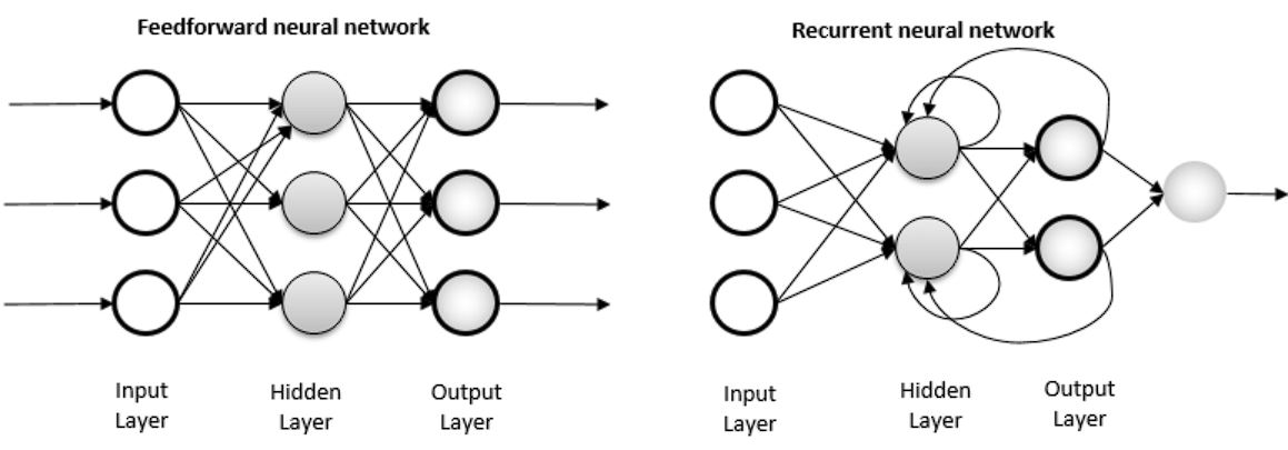
In a standard feed-forward neural network or Multi-Layer Perceptron, the data flows only in one direction, from the input layer, through the hidden layers, and to the output layer. There are no loops in the network, and the output of any layer does not affect that same layer in the future. Each input is independent and doesn’t affect the next input; in other words, there are no long-term dependencies.
In contrast, in an RNN model, the information cycles through a loop. When the model makes a prediction, it considers the current input and what it has learned from the previous inputs.
Weights
There are 3 different weights used in RNNs:
- Input-to-Hidden Weights (W_xh): These weights connect the input to the hidden state.
- Hidden-to-Hidden Weights (W_hh): These weights connect the previous hidden state to the current hidden state and are learned by the network.
- Hidden-to-Output Weights (W_hy): These weights connect the hidden state to the output.
Bias Vectors
Two bias vectors are used, one for the hidden state and the other for the output.
Activation Functions
The two functions used are tanh and ReLU, where tanh is used for the hidden state.
A single pass in the network looks like this:
At time step t, given input x_t and previous hidden state h_t-1:
- The network computes the intermediate value z_t using the input, previous hidden state, weights, and biases.
- It then applies the activation function tanh to z_t to get the new hidden state h_t
- The network then computes the output y_t using the new hidden state, output weights, and output biases.
This process is repeated for each time step in the sequence and the next letter or word is predicted in the sequence.
Backpropagation Through Time
A backward pass in a neural network is used to update the weights to minimize the loss. However, in RNNs, it is a little more complex than a standard feed-forward network, therefore, the standard backpropagation algorithm is customized to incorporate the recurrent nature of RNNs.
In a feed-forward network, backpropagation looks like this:
- Forward Pass: The model computes the activations and outputs of each layer, one by one.
- Backward Pass: Then it computes the gradients of the loss with respect to the weights and repeats the process for all the layers.
- Parameter Update: Update the weights and biases using the gradient descent algorithm.
However, in RNNs, this process is adjusted to incorporate the sequential data. To learn to predict the next word correctly, the model needs to learn what weights in the previous time steps led to the correct or incorrect prediction.
Therefore, an unrolling process is performed. Unrolling the RNNs means that for each time step, the entire RNN is unrolled, representing the weights at that particular time step. For example, if we have t time steps, then there will be t unrolled versions.
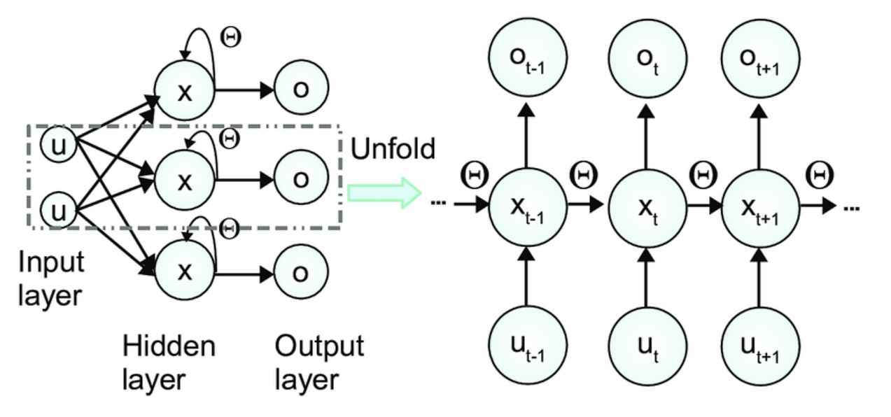
Once this is performed, the losses are calculated for each time step, and then the model computes the gradients of the loss for hidden states, weights, and biases, backpropagating the error through the unrolled network.
This pretty much explains the working of RNNs.
RNNs face serious limitations such as exploding and vanishing gradients problems, and limited memory. Combining all these limitations made training RNNs difficult. As a result, LSTMs were developed, that inherited the foundation of RNNs and combined with a few changes.
Sequence Model 2: Long Short-Term Memory Networks (LSTM)
LSTM networks are a special kind of RNN-based sequence model that addresses the issues of vanishing and exploding gradients and are used in applications such as sentiment analysis. As we discussed above, LSTM utilizes the foundation of RNNs and hence is similar to it, but with the introduction of a gating mechanism that allows it to hold memory over a longer period.
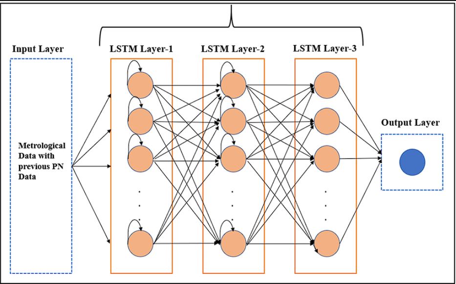
An LSTM network consists of the following components.
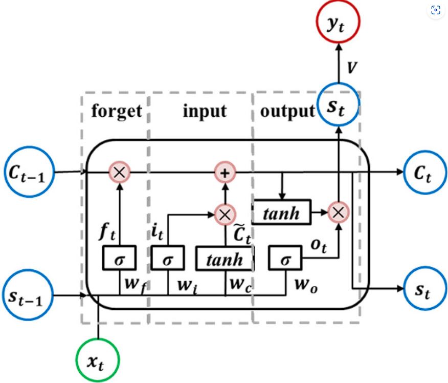
Cell State
The cell state in an LSTM network is a vector that functions as the memory of the network by carrying information across different time steps. It runs down the entire sequence chain with only some linear transformations, handled by the forget gate, input gate, and output gate.
Hidden State
The hidden state is the short-term memory in comparison cell state that stores memory for a longer period. The hidden state serves as a message carrier, carrying information from the previous time step to the next, just like in RNNs. It is updated based on the previous hidden state, the current input, and the current cell state.
LSTMs use three different gates to control information stored in the cell state.
Forget Gate Operation
The forget gate decides which information from the previous cell state should be carried forward and which must be forgotten. It gives an output value between 0 and 1 for each element in the cell state. A value of 0 means that the information is completely forgotten, while a value of 1 means that the information is fully retained.
This is decided by element-wise multiplication of the forget gate output with the previous cell state.
Input Gate Operation
The input gate controls which new information is added to the cell state. It consists of two parts: the input gate and the cell candidate. The input gate layer uses a sigmoid function to output values between 0 and 1, deciding the importance of new information.
The values output by the gates are not discrete; they lie on a continuous spectrum between 0 and 1. This is due to the sigmoid activation function, which squashes any number into the range between 0 and 1.
Output Gate Operation
The output gate decides what the next hidden state should be by deciding how much of the cell state is exposed to the hidden state.
Let us now look at how all these components work together to make predictions.
- At each time step t, the network receives an input x_t
- For each input, LSTM calculates the values of the different gates. Note that these are learnable weights, as with time the model gets better at deciding the value of all three gates.
- The model computes the Forget Gate.
- The model then computes the Input Gate.
- It updates the Cell State by combining the previous cell state with the new information, which is decided by the value of the gates.
- Then it computes the Output Gate, which decides how much information of the cell state needs to be exposed to the hidden state.
- The hidden state is passed to a fully connected layer to produce the final output
Sequence Model 3: Gated Recurrent Unit (GRU)
LSTM and Gated Recurrent Units are both types of Recurrent Networks. However, GRUs differ from LSTMs in the number of gates they use. GRU is simpler in comparison to LSTM and uses only two gates instead of using three gates found in LSTM.
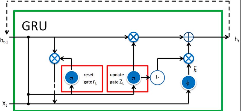
Moreover, GRU is simpler than LSTM in terms of memory, as it only utilizes the hidden state for memory. Here are the gates used in GRU:
- The update gate in GRU controls how much of the past information needs to be carried forward.
- The reset gate controls how much information in the memory it needs to forget.
- The hidden state stores information from the previous time step.
Sequence Model 4: Transformer Models
The transformer model has been quite a breakthrough in the world of deep learning and has brought the eyes of the world to itself. Various LLMs such as ChatGPT and Gemini from Google use the transformer architecture in their models.
Transformer architecture differs from the previous models we have discussed in its ability to give varying importance to different parts of the sequence of words it has been provided. This is known as the self-attention mechanism and is proven to be useful for long-range dependencies in texts.
Self-Attention Model
As we discussed above, self-attention is a mechanism that allows the model to give varying importance and extract important features in the input data.
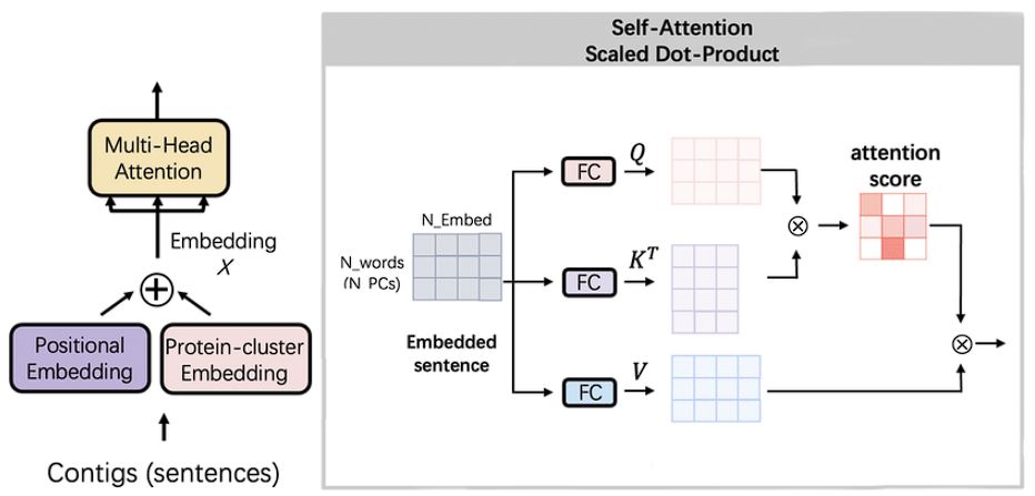
It works by first computing the attention score for each word in the sequence and derives their relative importance. This process allows the model to focus on relevant parts and gives it the ability to understand natural language, unlike any other model.
Architecture of the Transformer model
The key feature of the Transformer model is its self-attention mechanisms that allow it to process data in parallel rather than sequentially as in Recurrent Neural Networks (RNNs) or Long Short-Term Memory Networks (LSTMs).
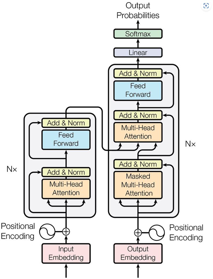
The Transformer architecture consists of an encoder and a decoder.
Encoder
The Encoder is composed of the same multiple layers. Each layer has two sub-layers:
- Multi-head self-attention mechanism.
- Fully connected feed-forward network.
The output of each sub-layer passes through a residual connection and a layer normalization before it is fed into the next sub-layer.
“Multi-head” here means that the model has multiple sets (or “heads”) of learned linear transformations that it applies to the input. This is important because it enhances the modeling capabilities of the network.
For example, the sentence: “The cat, which had already eaten, was full.” By having multi-head attention, the network will:
- Head 1 will focus on the relationship between “cat” and “eaten”, helping the model understand who did the eating.
- Head 2 will focus on the relationship between “eaten” and “full”, helping the model understand why the cat is full.
As a result of this, we can process the input and extract the context better in parallelly.
Decoder
The Decoder has a similar structure to the Encoder, but with one difference. Masked multi-head attention is used here. Its major components are:
- Masked Self-Attention Layer: Similar to the Self-Attention layer in the Encode,r but involves masking.
- Self-Attention Layer
- Feed-Forward Neural Network.
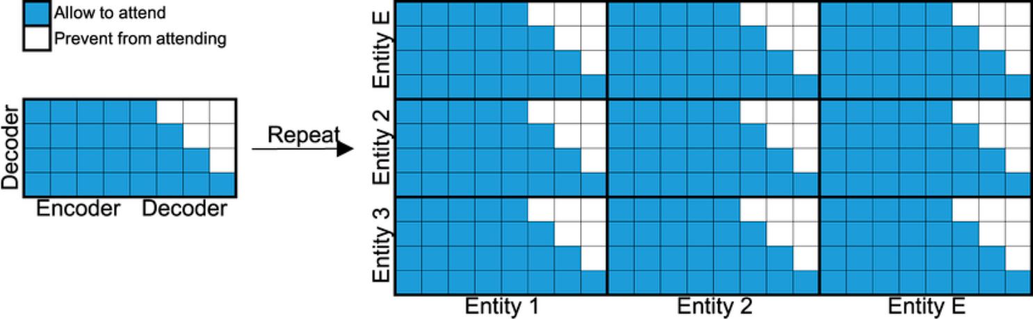
The “masked” part of the term refers to a technique used during training where future tokens are hidden from the model.
The reason for this is that during training, the whole sequence (sentence) is fed into the model at once, but this poses a problem, the model now knows what the next word is and there is no learning involved in its prediction. Masking out removes the next word from the training sequence provided, which allows the model to provide its prediction.
For example, let’s consider a machine translation task, where we want to translate the English sentence “I am a student” to French: “Je suis un étudiant”.
[START] Je suis un étudiant [END]
Here’s how the masked layer helps with prediction:
- When predicting the first word “Je”, we mask out (ignore) all the other words. So, the model doesn’t know the next words (it just sees [START]).
- When predicting the next word “suis”, we mask out the words to its right. This means the model can’t see “un étudiant [END]” for making its prediction. It only sees [START] Je.
Brief Recap of Sequence Models
In this blog, we looked into the different Convolution Neural Network architectures that are used for sequence modeling. We started with RNNs, which serve as a foundational model for LSTM and GRU. RNNs differ from standard feed-forward networks because of the memory features due to their recurrent nature, meaning the network stores the output from one layer and is used as input to another layer. However, training RNNs turned out to be difficult. As a result, we saw the introduction of LSTM and GRU which use gating mechanisms to store information for an extended time.
Finally, we looked at the Transformer machine learning model, an architecture that is used in notable LLMs such as ChatGPT and Gemini. Transformers differed from other sequence models because of their self-attention mechanism that allowed the model to give varying importance to part of the sequence, resulting in human-like comprehension of texts.
Read our blogs to understand more about the concepts we discussed here:
- Ensemble Learning: A Combined Prediction Model
- Scalable Pre-Training: Large Autoregressive Image Models
- Xception Model: Analyzing Depthwise Separable Convolutions
- Vision Language Models: Exploring Multimodal AI