Pandas: An Essential Python Data Analysis Library

Pandas is a free and open-source Python data analysis library specifically designed for data manipulation and analysis. It excels at working with structured data, often encountered in spreadsheets or databases. Pandas simplifies data cleaning by providing tools for tasks like sorting, filtering, and data transformation. It can effectively handle missing values, eliminate duplicates, and restructure your data to prepare it for analysis.

Beyond core data manipulation, pandas integrate seamlessly with data visualization libraries like Matplotlib and Seaborn. This integration empowers you to create plots and charts for visual exploration and a deeper understanding of the data.

Developed in 2008 by Wes McKinney for financial data analysis, pandas has grown significantly to become a versatile data science toolkit.

The creators of the Pandas library designed it as a high-level tool or building block to facilitate practical, real-world analysis in Python. The exceptional performance, user-friendliness, and seamless integration with other scientific Python libraries have made pandas a popular and capable tool for Data Science tasks.

About us: Viso Suite is the enterprise machine learning infrastructure that hands complete control of the entire application lifecycle to ML teams. With top-of-the-line security measures, ease of use, scalability, and accuracy, Viso Suite provides enterprises with 695% ROI in 3 years. To learn more, book a demo with our team.

The Core of Pandas Library

Pandas offers two primary data structures: Series (one-dimensional) and DataFrame (two-dimensional).

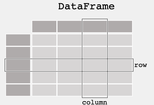
• DataFrame: A DataFrame is a two-dimensional, size-mutable data structure with labeled axes (rows and columns). They are easily readable and printable as a two-dimensional table.
• Series: A Series in pandas is a one-dimensional labeled array capable of holding data of various data types like integers, strings, floating-point numbers, Python objects, etc. Each element in the Series has a corresponding label, providing a way to access and reference data.

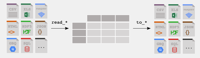
Moreover, Pandas allows for importing and exporting tabular data in various formats, such as CSV files, JSON, Exel files (.xlsx), and SQL databases.

Creating Data Frames and Series in Pandas

First, you need to set up your environment. You can use Jupyter Notebook or set up a custom environment.

1. Start by installing the Pandas library using: pip install pandas
2. Import pandas: import pandas as pd
3. Create DataFrame
4. Create Series

#creating dataframe
data = {'Name': ['Alice', 'Bob', 'Charlie'], 'Age': [25, 30, 28]}
df = pd.DataFrame(data)
print(df)

#Creating Series
fruits = ['apple', 'banana', 'orange']
series = pd.Series(fruits)
print(series)

Core Functionalities in Pandas

Pandas offers a wide range of functionalities to cater to the stages of the data processing pipeline for Machine Learning and Data Science tasks, moreover it is the most used in the collection of Python libraries for data analysis tasks. Some of the core functionalities include:

1. Data Selection and Indexing: It allows selecting and indexing data, either by label (loc), integer location (iloc), or a mixture of both.
2. Data Cleaning:  Identifying and handling missing data, duplicate entries, and data inconsistencies.
3. Data Transformation: Tasks such as pivoting, reshaping, sorting, aggregating, and merging datasets.
4. Data Filtering: Filtering methods to select subsets of data based on conditional criteria.
5. Statistical Analysis: Pandas provides functions to perform descriptive statistics, correlation analysis, and aggregation operations.
6. Time Series Analysis: With specialized time series functionalities, Pandas is well-equipped to handle date and time data, and perform date arithmetic, resampling, and frequency conversion.
7. Visualization: Creating plots and graphs of the data.

Data Selection and Indexing

Pandas provides several tools for selecting data from DataFrames using several methods.

Selecting rows and columns in Pandas can be done in several ways, depending on the specific requirements of your task. Here’s a guide to some of the most common methods using loc, iloc, and other techniques:

Using loc for Label-Based Selection

• Single column: df.loc[:, ‘column_name’]
• Multiple columns: df.loc[:, [‘column_name1’, ‘column_name2’]]
• Single row: df.loc[‘row_label’]
• Multiple rows: df.loc[[‘row_label1’, ‘row_label2’]]

Using iloc for Position-Based Selection

• Single column: df.iloc[:, 2] (selects the third column)
• Multiple columns: df.iloc[:, [1, 3]] (selects the second and fourth columns)
• Single row: df.iloc[4] (selects the fifth row)
• Multiple rows: df.iloc[[1, 3]] (selects the second and fourth rows)

Boolean Indexing

• Rows based on condition: df[df[‘column_name’] > value] (selects rows where the condition is True)
• Using loc with a condition: df.loc[df[‘column_name’] == ‘value’, [‘column1’, ‘column2’]]

import pandas as pd
import numpy as np
# Creating a sample DataFrame
data = {
    'Name': ['John', 'Anna', 'Peter', 'Linda'],
    'Age': [28, 34, 29, 32],
    'City': ['New York', 'Paris', 'Berlin', 'London'],
    'Salary': [68000, 72000, 71000, 69000]
}
df = pd.DataFrame(data)
# Using loc for label-based selection
multiple_columns_loc = df.loc[:, ['Name', 'Age']]
# Using iloc for position-based selection
multiple_columns_iloc = df.iloc[:, [0, 1]]
# Rows based on condition
rows_based_on_condition = df[df['Age'] > 30]
# Using loc with a condition
loc_with_condition = df.loc[df['City'] == 'Paris', ['Name', 'Salary']]

#output 
Using loc for Label-Based Selection
    Name  Age
0   John   28
1   Anna   34
2  Peter   29
3  Linda   32
Rows Based on Condition (Age > 30)
    Name  Age    City  Salary
1   Anna   34   Paris   72000
3  Linda   32  London   69000
Using loc with a Condition (City == 'Paris')
   Name  Salary
1  Anna   72000

Data Cleaning and Handling Missing Values

Importance of Data Cleaning

Real-world data often contains inconsistencies, errors, and missing values. Data cleaning is crucial to ensure the quality and reliability of your analysis. Here’s why it’s important:

• Improved Data Quality
• Enhanced Analysis
• Model Efficiency in ML

Missing values are data points that are absent or not recorded. They can arise due to various reasons like sensor malfunctions, user skipping fields, or data entry errors. Here are some common methods for handling missing values in pandas:

Identifying Missing Values

• Check for missing values: Use df.isnull() or df.isna() to check for missing values, which returns a boolean DataFrame indicating the presence of missing values.
• Count missing values: df.isnull().sum() to count the number of missing values in each column.

Handling Missing Values

• Remove missing values:
  • df.dropna() drops rows with any missing values.
  • df.dropna(axis=1) drops columns with any missing values.
• Fill missing values:
  • df.fillna(value) fills missing values with a specified value.
  • df[‘column’].fillna(df[‘column’].mean()) fills missing values in a specific column with the mean of that column.

Data Transformation

• Removing duplicates: df.drop_duplicates() removes duplicate rows.
• Renaming columns: df.rename(columns={‘old_name’: ‘new_name’}) to rename columns.
• Changing data types: df.astype({‘column’: ‘dtype’}) changes the data type of a column.
• Apply functions: df.apply(lambda x: func(x)) applies a function across an axis of the DataFrame.

# Sample data with missing values
data = {'Name': ['John', 'Anna', 'Peter', None],
        'Age': [28, np.nan, 29, 32],
        'City': ['New York', 'Paris', None, 'London']}
df = pd.DataFrame(data)
# Check for missing values
missing_values_check = df.isnull()
# Count missing values
missing_values_count = df.isnull().sum()
# Remove rows with any missing values
cleaned_df_dropna = df.dropna()
# Fill missing values with a specific value
filled_df = df.fillna({'Age': df['Age'].mean(), 'City': 'Unknown'})
# Removing duplicates (assuming df has duplicates for demonstration)
deduped_df = df.drop_duplicates()
# Renaming columns
renamed_df = df.rename(columns={'Name': 'FirstName'})
# Changing data type of Age to integer (after filling missing values for demonstration)
df['Age'] = df['Age'].fillna(0).astype(int)
missing_values_check, missing_values_count, cleaned_df_dropna, filled_df, deduped_df, renamed_df, df

#ouputs

Check for missing values
   Name    Age   City
0  False  False  False
1  False   True  False
2  False  False   True
3   True  False  False
Counting Missing Values
Name 1
Age 1
City 1
dtype: int64
Removing the missing values
 Name Age City
0 John 28.0 New York

DataFiltering and Statistical Analysis

Statistical analysis in Pandas involves summarizing the data using descriptive statistics, exploring relationships between variables, and performing inferential statistics. Common operations include:

• Descriptive Statistics: Functions like describe(), mean(),  and sum() provide summaries of the central tendency, dispersion, and shape of the dataset’s distribution.
• Correlation: Calculating the correlation between variables using corr(), to understand the strength and direction of their relationship.
• Aggregation: Using groupby() and agg() functions to summarize data based on categories or groups.

Data filtering in Pandas can be performed using boolean indexing in which it selects entries that meets a specific criteria ( for e.g. sales > 20)

# Sample data creation
sales_data = {
    'Product': ['Table', 'Chair', 'Desk', 'Bed', 'Chair', 'Desk', 'Table'],
    'Category': ['Furniture', 'Furniture', 'Office', 'Furniture', 'Furniture', 'Office', 'Furniture'],
    'Sales': [250, 150, 200, 400, 180, 220, 300]
}
sales_df = pd.DataFrame(sales_data)
inventory_data = {
    'Product': ['Table', 'Chair', 'Desk', 'Bed'],
    'Stock': [20, 50, 15, 10],
    'Warehouse_Location': ['A', 'B', 'C', 'A']
}
inventory_df = pd.DataFrame(inventory_data)
# Merging sales and inventory data on the Product column
merged_df = pd.merge(sales_df, inventory_df, on='Product')
# Filtering data 
filtered_sales = merged_df[merged_df['Sales'] > 200]
# Statistical Analysis
# Basic descriptive statistics for the Sales column
sales_descriptive_stats = merged_df['Sales'].describe()

#ouputs
Filtered Sales Data (Sales > 200):
  Product   Category  Sales  Stock Warehouse_Location
0   Table  Furniture    250     20                  A
3     Bed  Furniture    400     10                  A
5    Desk     Office    220     15                  C
6   Table  Furniture    300     20                  A
Descriptive Statistics for Sales:
count      7.000000
mean     242.857143
std       84.599899
min      150.000000
25%      190.000000
50%      220.000000
75%      275.000000
max      400.000000
Name: Sales, dtype: float64

Data Visualization

Pandas is primarily focused on data manipulation and analysis, however, it offers basic plotting functionalities to get you started with data visualization.

Data visualization in Pandas is built on top of the matplotlib library, making it easy to create basic plots from DataFrames and Series without needing to import matplotlib explicitly. This functionality is accessible through the .plot() method and provides a quick and straightforward way to visualize your data for analysis.

Pandas AI

PandasAI is a third-party library built on top of the popular Pandas library for Python, that simplifies data analysis for Data Scientists and inexperienced coders. It leverages generative AI techniques and machine learning algorithms to enhance data analysis capabilities for the pandas framework, helping with machine learning modeling. It allows users to interact with their data through natural language queries instead of writing complex pandas code. Here is the GitHub repo.

Additionally, it can be used to generate summaries, visualize the data, handle missing values, and feature engineering, all of it using just prompts.

To install it, you just have to use pip install pandasai.

Here is an example code for its usage.

import os
import pandas as pd
from pandasai import Agent
# Sample DataFrame
sales_by_country = pd.DataFrame({
    "country": ["United States", "United Kingdom", "France", "Germany", "Italy", "Spain", "Canada", "Australia", "Japan", "China"],
    "sales": [5000, 3200, 2900, 4100, 2300, 2100, 2500, 2600, 4500, 7000]
})
# By default, unless you choose a different LLM, it will use BambooLLM.
# You can get your free API key signing up at https://pandabi.ai (you can also configure it in your .env file)
os.environ["PANDASAI_API_KEY"] = "YOUR_API_KEY"
agent = Agent(sales_by_country)
agent.chat('Which are the top 5 countries by sales?')

output: China, United States, Japan, Germany, Australia

agent.chat(
    "What is the total sales for the top 3 countries by sales?"
)
output: The total sales for the top 3 countries by sales is 16500.

Use Cases of Pandas AI

Pandas library is extensively used not just by data scientists, but also in several other fields such as:

• Scientific Computing: Pandas can be combined with other libraries (NumPy) to perform linear algebra operations. You can perform Basic Vector and Matrix Operations, solve linear equations, and other mathematical tasks. Moreover, scikit-learn library is extensively used in combination with Pandas.
• Statistical Analysis: Pandas provides built-in functions for various statistical operations. You can calculate descriptive statistics like mean, median, standard deviation, and percentiles for entire datasets or subsets.
• Machine Learning: Pandas facilitates feature engineering, a crucial step in machine learning. It enables data cleaning, transformation, and selection to create informative features that power accurate machine-learning models.
• Time Series: Industries like retail and manufacturing use time series analysis to identify seasonal patterns, predict future demand fluctuations, and optimize inventory management. Pandas library is well-suited for working with time series data. Features like date-time indexing, resampling, and frequency conversion, all assist with managing time series data.
• Financial Analysis: Pandas is used to analyze vast financial datasets, and track market trends. Its data manipulation capabilities streamline complex financial modeling and risk analysis.