Optical flow quantifies the motion of objects between consecutive frames captured by a camera. These algorithms attempt to capture the apparent motion of brightness patterns in the image. It is an important subfield of computer vision, enabling machines to understand scene dynamics and movement.
Optical Flow Concept
The concept of optical flow dates back to the early works of James Gibson in the 1950s. Gibson introduced the concept in the context of visual perception. Researchers didn’t start studying and using optical flow until the 1980s when computational tools were introduced.
A significant milestone was the development of the Lucas-Kanade method in 1981. This provided a foundational algorithm for estimating optical flow in a local window of an image. The Horn-Schunck algorithm followed soon after, introducing a global approach to optical flow estimation across the entire image.
Optical flow estimation relies on the assumption that the brightness of a point is constant over short periods. Mathematically, this is expressed through the optical flow equation, Ixvx+Iyvy+It=0.
- Ix and Iy reflect the spatial gradients of the pixel intensity in the x and y directions, respectively
- It is the temporal gradient
- vx and vyare the flow velocities in the x and y directions, respectively.
More recent breakthroughs involve leveraging deep learning models like FlowNet, FlowNet 2.0, and LiteFlowNet. These models transformed optical flow estimation by significantly improving accuracy and computational efficiency. This is largely because of the integration of Convolutional Neural Networks (CNNs) and the availability of large datasets.
Even in settings with occlusions, optical flow techniques nowadays can accurately anticipate complicated patterns of apparent motion.
Techniques and Algorithms for Optical Flow
Different types of optic flow algorithms, each with a unique way of calculating the pattern of motion, led to the evolution of computational approaches. Traditional algorithms like the Lucas-Kanade and Horn-Schunck methods laid the groundwork for this area of computer vision.
The Lucas-Kanade Method
This method caters to use cases with a sparse feature set. It operates on the assumption that flow is locally smooth, applying a Taylor-series approximation to the image gradients. You can thereby solve an optical flow equation, which typically involves two unknown variables for each point in the feature set. This method is highly efficient for tracking well-defined corners and textures often, as identified by the Shi-Tomasi corner detection or the Harris corner detector.
The Horn-Schunck Algorithm
This algorithm is a dense optical flow technique. It takes a global approach by assuming smoothness in the optical flow across the entire image. This method minimizes a global error function and can infer the flow for every pixel. It offers more detailed structures of motion at the cost of higher computational complexity.
However, novel deep learning algorithms have ushered in a new era of optical flow algorithms. Models like FlowNet, LiteFlowNet, and PWC-Net use CNNs to learn from vast datasets of images. This enables the prediction with greater accuracy and robustness, especially in challenging scenarios. For example, in scenes with occlusions, varying illumination, and complex dynamic textures.
To illustrate the differences among these algorithms, consider the following comparative table that outlines their performance in terms of accuracy, speed, and computational requirements:
| Algorithm | Accuracy | Speed (FPS) | Computational Requirements |
|---|---|---|---|
| Lucas-Kanade | Moderate | High | Low |
| Horn-Schunck | High | Low | High |
| FlowNet | High | Moderate | Moderate |
| LiteFlowNet | Very High | Moderate | Moderate |
| PWC-Net | Very High | High | High |
Traditional techniques such as Lucas-Kanade and Horn-Schunck are foundational and should not be discounted. However, they generally can’t compete with the accuracy and robustness of deep learning approaches. Deep learning methods, while powerful, often require substantial computational resources. This means they might not be as suitable for real-time applications.
In practice, the choice of algorithm depends on the specific application and constraints. The speed and low computational load of the Lucas-Kanade method may be more apt for a mobile app. The detailed output of a dense approach, like Horn-Shunck, may be more suitable for an offline video analysis task.
Optical Flow in Action – Use Cases and Applications
Today, you’ll find applications of optical flow technology in a variety of industries. It’s becoming increasingly important for smart computer vision technologies that can interpret dynamic visual information quickly.
Automotive: ADAS and Autonomous Driving, and Traffic Monitoring
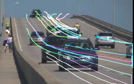
Optical flow serves as a cornerstone technology for Advanced Driver Assistance Systems (ADAS). For instance, Tesla’s Autopilot uses these algorithms in its suite of sensors and cameras to detect and track objects. It assists in estimating the velocity of moving objects relative to the car as well. These capabilities are crucial for collision avoidance and lane tracking.
Surveillance and Security: Crowd Monitoring and Anomalous Behavior Detection
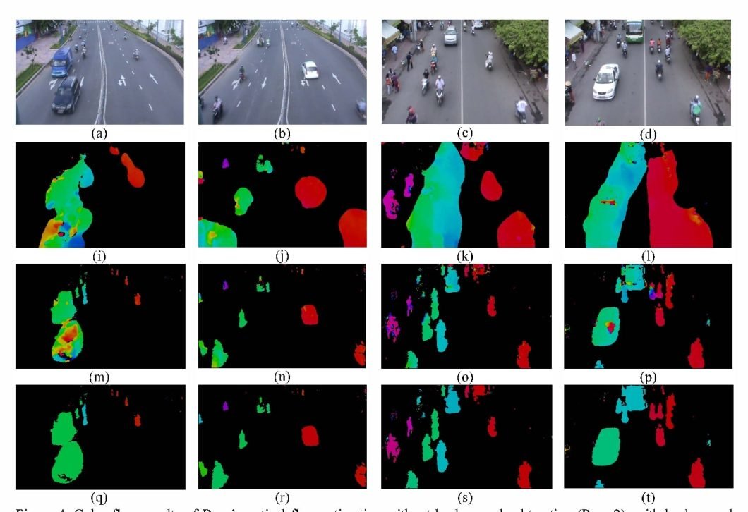
Optical flow aids in crowd monitoring by analyzing the flow of people to help detect patterns or anomalies. When looking at uses of computer in airports or shopping centers, for example, it can flag unusual movements and alert security. It could be something as simple (but hard to see) as an individual moving against the crowd. Events like the FIFA World Cup often use it to help monitor crowd dynamics for safety purposes.
Sports Analytics: Motion Analysis for Performance Improvement and Injury Prevention
By analyzing the flow of players across the field, teams can optimize training and strategies for improved athletic output. Catapult Sports, a leader in athlete analytics, leverages optical flow to track player movements. This provides coaches with data to enhance performance and reduce injury risks.
Robotics: Navigation and Object Avoidance
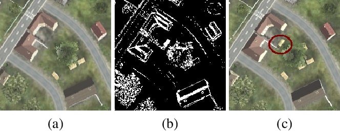
Drone technology companies, like Da-Jiang Innovations (DJI), use visual sensors to stabilize flight and avoid obstacles. It also analyzes surface patterns, helping drones maintain position by calculating their motion relative to the ground. This helps ensure safe navigation, even without GPS systems.
Film and Video Production: Visual Effects, Motion Tracking, and Scene Reconstruction
Filmmakers use optical flow to create visual effects and in post-production editing. The visual effects team for the movie “Avatar” used these techniques for motion tracking and scene reconstruction. This allows for the seamless integration of Computer-generated Imagery (CGI) with live-action footage. It can facilitate the recreation of complex dynamic scenes to provide realistic and immersive visuals.
Optical Flow Practical Implementation
There are various ways of implementing optical flow in applications, ranging from AI software to hardware integration. As an example, we’ll look at a typical integration process using the popular OpenCV optical flow algorithm.
OpenCV (Open Source Computer Vision Library) is an extensive library offering a range of real-time computer vision capabilities. This includes utilities for image and video analysis, feature detection, and object recognition. Known for its versatility and performance, OpenCV is widely used in academia and industry for rapid prototyping and deployment.
Applying the Lucas-Kanade Method in OpenCV
- Environment Setup: Install OpenCV using package managers like pip for Python with the command
pip install opencv-python. - Read Frames: Capture video frames using OpenCV’s
VideoCaptureobject. - Preprocess Frames: Convert frames to grayscale
cvtColorfor processing, as optical flow requires single-channel images. - Feature Selection: Use
goodFeaturesToTrackfor selecting points to track or pass a predefined set of points. - Lucas-Kanade Optical Flow: Call
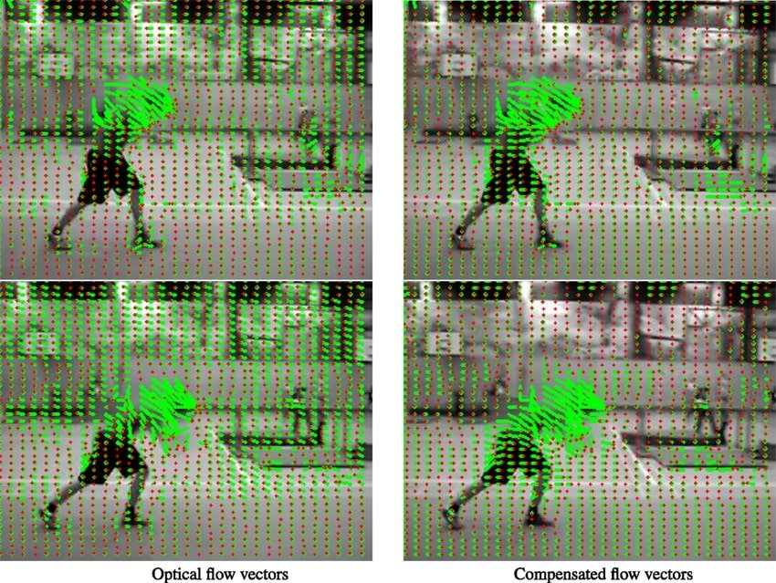
calcOpticalFlowPyrLKto estimate the optical flow between frames. - Visualize Flow: Draw the flow vectors on images to verify the flow’s direction and magnitude.
- Iterate: Repeat the process for subsequent frame pairs to track motion over time.
Integrating Optical Flow into Hardware Projects
An example can include drones for real-time motion tracking:
- Sensor Selection: Choose an optical flow sensor compatible with your hardware platform, like the PMW3901 for Raspberry Pi.
- Connectivity: Connect the sensor to your hardware platform’s GPIO pins or use an interfacing module if necessary.
- Driver Installation: Install the necessary drivers and libraries to interface with the sensor.
- Data Acquisition: Write code to read the displacement data from the sensor, representing the optical flow.
- Application Integration: Feed the sensor data into your application logic to use the optical flow for tasks like navigation or obstacle avoidance.
Performance Optimizations
You may also want to consider the following to optimize performance for optical flow applications:
- Quality of Features: Ensure selected points are well-distributed and trackable over time.
- Parameter Tuning: Adjust the parameters of the function to balance between speed and accuracy.
- Pyramid Levels: Use image pyramids to track points at different scales to account for changes in motion and scale.
- Error Checking: Implement error checks to filter out unreliable flow vectors.
Challenges and Limitations
Occlusions, illumination changes, and texture-less regions still present a significant challenge to the accuracy of optical flow systems. Predictive models that estimate the motion of occluded areas based on surrounding visible elements can improve the outcomes. Adaptive algorithms that can normalize light variations may also assist in compensating for illumination changes. Optical flow for sparsely textured regions can benefit from integrating spatial context or higher-level cues to infer motion.
Another challenge commonly faced is known as the “two unknown problem.” This arises due to having more variables than equations, making the calculations underdetermined. By assuming flow consistency over small windows, you can mitigate this issue by allowing for the aggregation of information to solve for the unknowns. Other advanced methods may further refine estimates using iterative regularization techniques.
Current models and algorithms may struggle in complex environments with rapid movements, diverse object scales, and 3D depth variations. One solution is the development of multi-scale models that operate across different resolutions. Another is the integration of depth information from stereo vision or LiDAR, for example, to enhance 3D scene interpretation.