In the following, we will guide you step-by-step through the concept of an artificial neural network, how it works, and the elements it is based on. Some degree of prior Python and artificial intelligence knowledge helps understand the technical terminology. If you are new to AI, we recommend that you read our easy-to-understand guide (What is deep learning?).
An Introduction to ANNs
The Artificial Neurons
The very first step to grasping what an artificial neural network does is to understand the neuron. Neural networks in computer science mimic actual human brain neurons, hence the name “neural” network.
Neurons have branches coming out of them from both ends, called dendrites. One neuron can’t do much, but when thousands of neurons connect and work together, they can process complex actions and concepts. A computer node works in the same way a human neuron does and replicates real neurons.
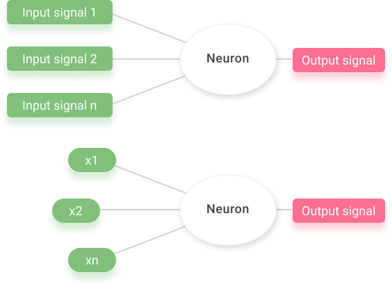
For us, input values like the signals in green above come from our senses. The green signifies an input layer. Layers are a common theme in neural networks because, like the human brain, one layer is relatively weak while many are strong. What we hear, smell, touch, or whatever it may be, gets processed as an input layer and then sent out as an output layer.
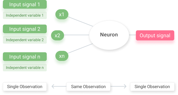
For our digital neuron, independent values (input signals) get passed through the “neuron” to generate a dependent value (output signal). This is considered to be “neuron activation.” These independent variables in one layer are just a row of data for one single observation.
For example, in the context of a neural network problem, one input layer would signify one variable – maybe the age or gender (independent variable) of a person whose identity (dependent) we are trying to figure out.
This neural network is then applied as many times as the number of data points per independent variable. So what would be the output value, since we now know what the input value signifies? Output values can be continuous, binary, or categorical variables.
They just have to correspond to the one row you input as the independent variables. In essence, one type of independent variable corresponds to one type of output variable. Those output variables can be the same for different rows, while the input variables cannot.
Weights and Activation
The next thing you need to know is what goes in the synapses. The synapses are those lines connecting the neuron to the input signals. Weights are assigned to all of them. Weights are crucial to artificial neural networks because they let the networks “learn.”
The weights decide which input signals are not important, which ones get passed along, and which don’t.
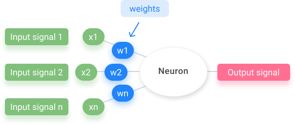
What happens in the neuron? The first step is to sum all the values passed through. In other words, it takes the weighted sum of all the input values. It then applies an activation function. Activation functions are just functions applied to the weighted sum.
Depending on the outcome of the applied function, the neuron will either pass on a signal or won’t pass it on.

Most machine learning algorithms can be done in this type of form, with an array of input signals going through an activation function (which can be anything: logistic regression, polynomial regression, etc.), and an output signal at the end.
How do Artificial Neural Networks Learn?
In general, there are two ways of training a model to learn from itself.
- Hard coding: you go through every case and possibility and create the algorithm yourself.
- Neural networks: You create an environment where your model can learn by giving inputs and outputs, and you are given a pre-programmed algorithm.
We’re going to be learning about neural networks and how they actually learn from themselves. We are not going to be giving other rules to the network, instead, we’ll be relying on the pre-programmed algorithm to do the bulk of the mathematical work for us.
This is common practice when making machine learning models. The neural network we see below is known as a single-layer feedforward neural network.
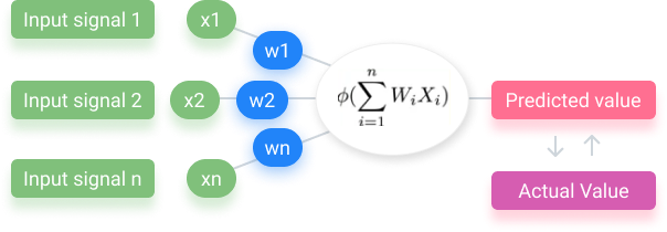
To learn, the predicted value created by the process above is compared to the actual value, which is given as a test variable. Some part of a dataset is divided so that it is just for the process to test itself with. The model keeps checking itself against the actual value, and makes modifications with each correct or incorrect value. It does this by calculating the cost function.
Cost Function to Determine Performance
In machine learning, cost functions are used to estimate how successfully models are performing (model performance evaluation). The cost function is ½ of the difference between the predicted value and the accurate value squared.
C = 1/2 (predicted – actual) ^ 2
The cost function’s purpose is to calculate the error we get from our prediction. Our goal is to minimize the cost function. The smaller the output of the cost function, the closer the predicted value is to the actual value.
Once we’ve compared, we feed this information back into the neural network. As we feed the results of the cost function into the neural network, it updates the weights. This entails that the only thing we’d really have control over in the neural network set up is the weights.
Artificial Neural Networks In Practice
Let’s consider the entirety of neural networks and how they function altogether by looking at an example problem. In this task, we are tasked with creating a machine learning model that can accurately predict whether or not an animal is a dog or cat based on its nose width and ear length. This model will be able to provide us with the percent probability of what type of animal the given data corresponds to.
This may not be a practical machine learning model, it is just an example. Here, X independent variables are shown in green and consist of ear length in cm and nose width in cm, while the Y variable is blue and reflects animal type.
The data tables below are a sample training and testing dataset, where we have 100 training data points and 10 testing – evenly split between dogs and cats (50 dog and 50 cat data points for training, 5 dog and 5 cat data points for testing).
We chose a 90-10 split because it is common practice to put away 80-90% of a given dataset to test with.
Training Dataset

Testing Dataset

We have 90 ID numbers, meaning the network observes 90 animals for training. We have ten data points to check our accuracy against. The neural network will apply to the 90 data points in our testing set. That’s why we can see multiple instances of the neural network above.
Since we have 90 data points, the neural network will iterate over the data points once each, making for 90 total iterations for this one neural network. This would cause 90 separate predicted and accurate values.
Analysis of Practice Neural Network
Each output is the predicted animal type for a set of ear length and nose width. It creates an epoch after the cost function makes an accuracy rate out of all the outputs. An epoch is when we go through the whole dataset, and the artificial neural network uses all of the rows to train.
Each epoch produces a total accuracy rate, which is calculated by a cost function that determines how much the weights change in the future. We update them according to whichever neural network algorithm we are using, so we do not manually change these weights.
In theory, each consecutive epoch should be more accurate than the last. The accuracy of a chosen epoch is the accuracy of that model. Each epoch signifies a unique model. After calculating the epoch accuracy rate, the model is ready to use.
In summation, there are four essential steps: setup, dataset, cost function, and epochs. This should be all you need to know to understand the basic form in which a machine-learning model works.
Challenges of Artificial Neural Networks
In practice, there is a limit to how many additional learning iterations can improve the model’s accuracy. At some point, the model will be overtrained and lose accuracy again. This effect is called “overtraining”; it occurs when the model becomes “over-familiar” with the data, resulting in a decrease in its ability to generalize and adapt to new data (unseen images).
The main challenges of training Artificial Neural Networks include optimizing hyperparameters, dealing with large datasets and long training times, avoiding overfitting and underfitting, understanding different optimization algorithms, and dealing with high-dimensional input data.
What’s Next for Artificial Neural Networks?
Machine learning is an ever-growing field of artificial intelligence. More sophisticated neural network architectures contain a set of multiple, sequential layers to increase the algorithm’s accuracy; they are called Deep Neural Networks.
Explore other articles about related topics to learn more about machine learning and deep learning with practical applications:
- Learn about analyzing machine learning model performance
- An easy-to-understand guide to Deep Reinforcement Learning
- Read about the differences between ANN and CNN models
- Check out our software platform for visual AI applications
- Landmark ruling in a case about IP Protection of ANNs for music recommendation
- An Introduction to Natural Language Processing (NLP)
- What are Convolutional Neural Networks (CNNs)?
