
Computer vision has rapidly become an essential component of modern technology, transforming industries such as retail, logistics, healthcare, robotics, and autonomous vehicles. As computer vision models continue to evolve, it’s crucial to evaluate their performance accurately and efficiently.
Key Performance Metrics
To evaluate a computer vision model, we need to understand several key performance metrics. After we introduce the key concepts, we will provide a list of when to use which performance measure.
Precision
Precision is a performance measure that quantifies the accuracy of a model in making positive predictions. It is defined as the ratio of true positive predictions (correctly identified positive instances) to the sum of true positives and false positives (instances that were incorrectly identified as positive).
The formula to calculate Precision is:
Precision = True Positives (TP) / (True Positives (TP) + False Positives (FP))
Precision is important when the cost of false positives is high or when the goal is to minimize false detections. The metric measures the proportion of correct positive predictions. This helps to evaluate how well the model discriminates between relevant and irrelevant objects in analyzed images.
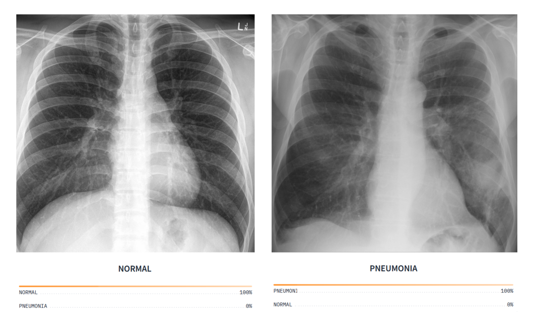
In computer vision tasks such as object detection, image segmentation, or facial recognition, Precision provides valuable insight into the model’s ability to correctly identify and localize target objects or features while minimizing false detections.

Recall
Recall, also known as Sensitivity or True Positive Rate, is a key metric in computer vision model evaluation. It is defined as the proportion of true positive predictions (correctly identified positive instances) among all relevant instances (the sum of true positives and false negatives, which are positive instances that the model failed to identify).
Therefore, the formula to calculate Recall is:
Recall = True Positives (TP) / (True Positives (TP) + False Negatives (FN))
The importance of Recall lies in its ability to measure the model’s capability to detect all positive cases, making it a critical metric in situations where missing positive instances can have significant consequences. Recall quantifies the proportion of positive instances that the model successfully identified. This provides insights into the model’s effectiveness in capturing the complete set of relevant objects or features in the analyzed images.
For example, in the context of a security system, Recall represents the proportion of actual intruders detected by the system. A high Recall value is desirable as it indicates that the system is effective in identifying potential security threats, minimizing the risk of undetected intrusions.

In other computer vision use cases where the cost of false negatives is high, such as medical imaging for AI diagnosis or anomaly detection, Recall serves as an essential metric to evaluate the model’s performance.
F1 Score
The F1 score is a performance metric that combines Precision and Recall into a single value, providing a balanced measure of a computer vision model’s performance. It is defined as the harmonic mean of Precision and Recall, calculated as follows:
Here is the formula to calculate the F1 Score:
F1 Score = 2 * (Precision * Recall) / (Precision + Recall)
The importance of the F1 score stems from its usefulness in scenarios with uneven class distributions or when false positives and false negatives carry different costs. By considering both Precision (the accuracy of positive predictions) and Recall (the ability to identify all positive instances), the F1 score offers a comprehensive evaluation of a model’s performance, particularly when the balance between false positives and false negatives is crucial.
For instance, in a medical imaging system, the F1 score helps determine the model’s overall effectiveness in detecting and diagnosing specific conditions. A high F1 score indicates that the model is successful in accurately identifying relevant features while minimizing both false positives (e.g., healthy tissue mistakenly flagged as abnormal) and false negatives (e.g., a condition that goes undetected).
In such applications, the F1 score serves as a valuable metric to ensure that the computer vision model performs optimally and minimizes potential risks associated with misdiagnosis or missed diagnosis.
Accuracy
Accuracy is a fundamental performance metric used in computer vision model evaluation. It is defined as the proportion of correct predictions (both true positives and true negatives) among all instances in a given dataset. In other words, it measures the percentage of instances that the model has classified correctly, considering both positive and negative classes.
This is the formula to calculate model accuracy:
Accuracy = (True Positives (TP) + True Negatives (TN)) / (True Positives (TP) + False Positives (FP) + True Negatives (TN) + False Negatives (FN))
The importance of accuracy stems from its ability to provide a straightforward measure of the model’s overall performance. It gives a general idea of how well the model performs on a given task, such as object detection, image classification, or segmentation.
However, accuracy may not be suitable in situations with significant class imbalances, as it can give a misleading impression of the model’s performance. In such cases, the model might perform well on the majority class but poorly on the minority class, leading to a high accuracy that doesn’t accurately reflect the model’s effectiveness in identifying all classes.
For example, in an image classification system, accuracy indicates the proportion of images that the model has classified correctly. A high accuracy value suggests that the model is effective in assigning the correct labels to images across all classes.
It is important to consider other performance metrics, such as Precision, Recall, and F1 score, to obtain a more comprehensive understanding of the model’s performance. This is especially the case when dealing with imbalanced datasets or scenarios with varying costs for different types of errors.
Intersection over Union (IoU)
Intersection over Union (IoU), also known as the Jaccard index, is a performance metric commonly used in computer vision model evaluation. It is particularly important for object detection and localization tasks. IoU is defined as the ratio of the area of overlap between the predicted bounding box and the ground truth bounding box to the area of their union.
In simple terms, IoU measures the degree of overlap between the model’s prediction and the actual target, expressed as a value between 0 and 1, with 0 indicating no overlap and 1 representing a perfect match.
The formula for Intersection over Union (IoU) is:
IoU = Area of Intersection / Area of Union
The importance of IoU lies in its ability to assess the localization accuracy of the model, capturing both the detection and positioning aspects of an object in an image. By quantifying the degree of overlap between the predicted and ground truth bounding boxes, IoU provides insights into the model’s effectiveness in identifying and localizing objects with precision.
For example, in a self-driving car’s object detection system, IoU measures how well the machine learning model can accurately detect and localize other vehicles, pedestrians, and obstacles in the car’s environment.
A high IoU value indicates that the model is successful in identifying objects and accurately estimating their position in the scene, which is essential for safe and efficient autonomous navigation. This is why the IoU performance metric is suitable for evaluating and improving computer vision model accuracy and performance of object detection tasks in real-world applications.

Mean Absolute Error (MAE)
Mean Absolute Error (MAE) is a metric used to measure the performance of ML models, such as those used in computer vision, by quantifying the difference between the predicted values and the actual values. MAE is the average of the absolute differences between the predictions and the true values.
MAE is calculated by taking the absolute difference between the predicted and true values for each data point, and then averaging these differences over all data points in the dataset. Mathematically, the formula for MAE is:
Mean Absolute Error (MAE) = (1/n) * Σ |Predicted Value - True Value|
where n is the number of data points in the dataset.
MAE helps assess the accuracy of a computer vision model by providing a single value that represents the average error in the model’s predictions. Lower MAE values indicate better model performance.
Since MAE is an absolute error metric, it is easier to interpret and understand compared to other metrics like mean squared error (MSE). Unlike MSE, which squares the differences and gives more weight to larger errors, MAE treats all errors equally, making it more robust to data outliers.
Mean Absolute Error can be used to compare different models or algorithms and to fine-tune hyperparameters. By minimizing MAE during training, a model can be optimized for better performance on unseen data.
Model Performance Evaluation Techniques
Several evaluation techniques help better understand ML model performance:
Confusion Matrix
A confusion matrix is a valuable tool for evaluating the performance of classification models, including those used in computer vision tasks. It is a table that displays the number of true positive (TP), true negative (TN), false positive (FP), and false negative (FN) predictions made by the model. These four components show how the instances have been classified across the different classes.
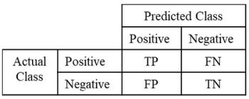
True Positives (TP) are instances correctly identified as positive, and True Negatives (TN) are instances correctly identified as negative. False Positives (FP) represent instances that were incorrectly identified as positive, while False Negatives (FN) are instances that were incorrectly identified as negative.
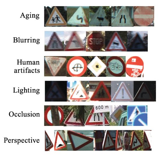
Visualizing the confusion matrix as a heatmap can make it easier to interpret the model’s performance. In a heatmap, each cell’s color intensity represents the number of instances for the corresponding combination of predicted and actual classes. This visualization helps quickly identify patterns and areas where the model may be struggling or excelling.
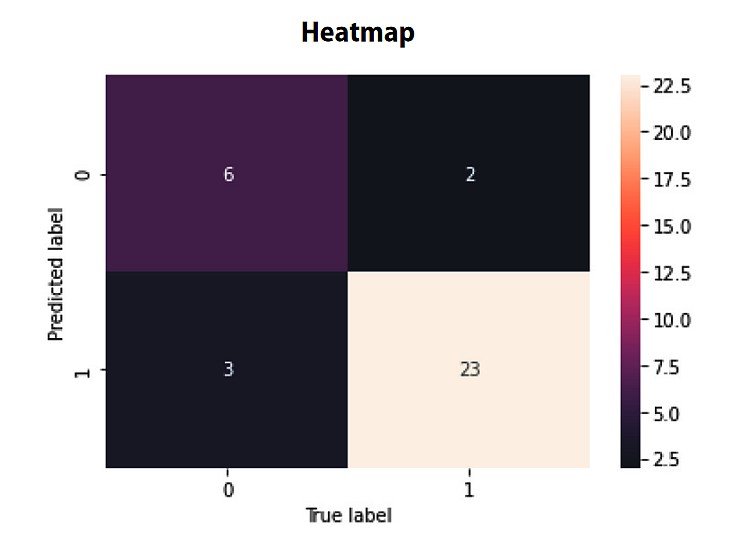
In a real-world example, such as a traffic sign recognition system, a confusion matrix can help identify which signs and situations lead to misclassification. By analyzing the matrix, developers can understand the model’s strengths and weaknesses to re-train the model for specific sign classes and challenging situations.
Receiver Operating Characteristic (ROC) Curve
The Receiver Operating Characteristic (ROC) curve is a performance metric used in computer vision model evaluation, primarily for classification tasks. It is defined as a plot of the true positive rate (sensitivity) against the false positive rate (1-specificity) for different classification thresholds.
By illustrating the trade-off between sensitivity and specificity, the ROC curve provides insights into the model’s performance across a range of thresholds.
To create the ROC curve, the classification threshold is varied, and the true positive rate and false positive rate are calculated at each threshold. The curve is generated by plotting these values, allowing for visual analysis of the model’s performance in distinguishing between positive and negative instances.
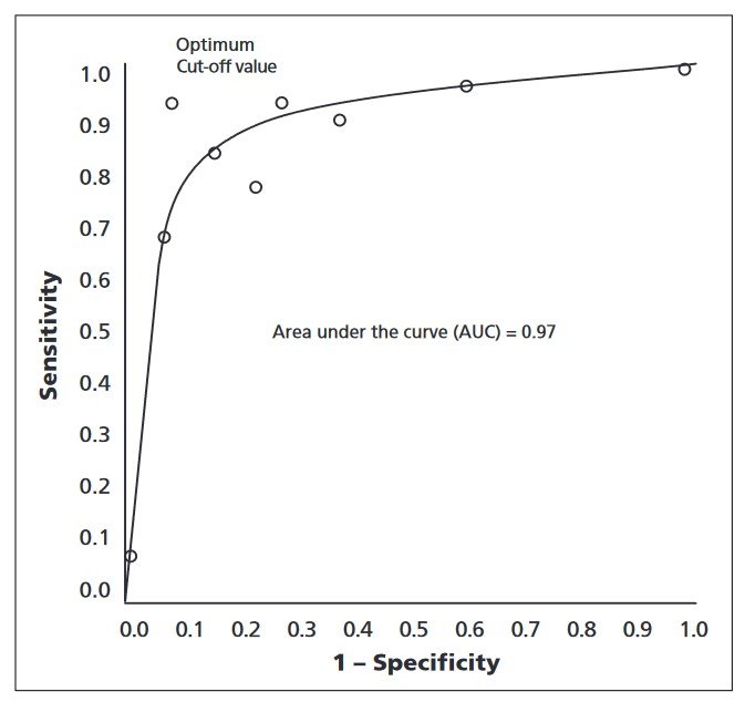
The Area Under the Curve (AUC) is a summary metric derived from the ROC curve, representing the model’s performance across all thresholds. A higher AUC value indicates a better-performing model, as it suggests that the model can effectively discriminate between positive and negative instances at various thresholds.
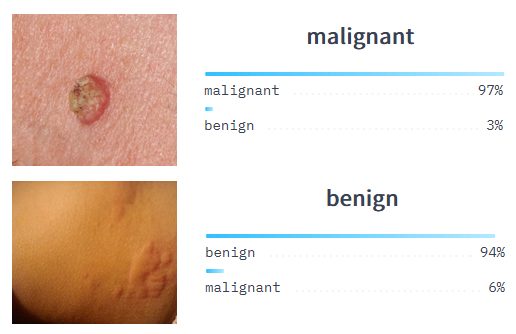
In real-world applications, such as a cancer detection system, the ROC curve can help identify the optimal threshold for classifying whether a tumor is malignant or benign. The curve helps to determine the best threshold that balances the need to correctly identify malignant tumors (high sensitivity) while minimizing false positives and false negatives.
Precision-Recall Curve
The Precision-Recall Curve is a performance evaluation method that shows the tradeoff between Precision and Recall for different classification thresholds. It helps visualize the trade-off between the model’s ability to make correct positive predictions (precision) and its capability to identify all positive instances (Recall) at varying thresholds.
To plot the curve, the classification threshold is varied, and Precision and Recall are calculated at each threshold. The curve represents the model’s performance across the entire range of thresholds, illustrating how precision and Recall are affected as the threshold changes.
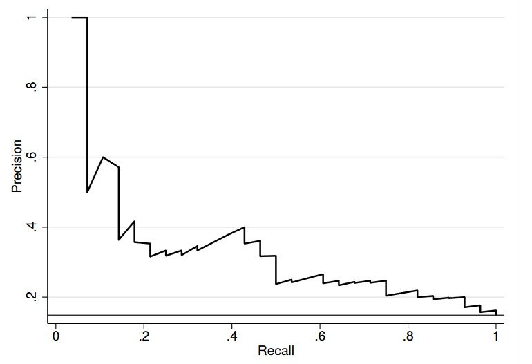
Average Precision (AP) is a summary metric that quantifies the model’s performance across all thresholds. A higher AP value indicates a better-performing model, reflecting its ability to achieve high Precision and Recall simultaneously. AP is particularly useful for comparing the performance of different models or tuning model parameters to achieve optimal performance.
A real-world example of the practical application of the Precision-Recall Curve can be found in spam detection systems. By analyzing the curve, developers can determine the optimal threshold for classifying emails as spam, while balancing false positives (legitimate emails marked as spam) and false negatives (spam emails that are not detected).
Dataset Considerations
Evaluating a computer vision model also requires careful consideration of the dataset:
Training and Validation Dataset Split
Training and Validation Dataset Split is a crucial step in developing and evaluating computer vision models. Dividing the dataset into separate subsets for training and validation helps estimate the model’s performance on unseen data. It also helps to address overfitting, ensuring that the ML model generalizes well to new data.
The three data sets – training, validation, and test sets – are essential components of the machine learning model development process:
- Training Set: A collection of labeled data points used to train the model, adjusting its parameters and learning patterns and features.
- Validation Set: A separate dataset for evaluating the model during development, used for hyperparameter tuning and model selection without introducing bias from the test set.
- Test Set: An independent dataset for assessing the model’s final performance and generalization ability on unseen data.
Splitting machine learning datasets is important to avoid training the model on the same data it is evaluated on. This would lead to a biased and overly optimistic estimation of the model’s performance. Commonly used split ratios for dividing the dataset are 70:30, 80:20, or 90:10, where the larger portion is used for training and the smaller portion for validation.
There are several techniques for splitting the data:
- Random sampling: Data points are randomly assigned to either the training or validation set, maintaining the overall data distribution.
- Stratified sampling: Data points are assigned to the training or validation set while preserving the class distribution in both subsets, ensuring that each class is well-represented.
- K-fold cross-validation: The dataset is divided into k equal-sized subsets, and the model is trained and validated k times, using each subset as the validation set once and the remaining subsets for training. The final performance is averaged over the k iterations.
Data Augmentation
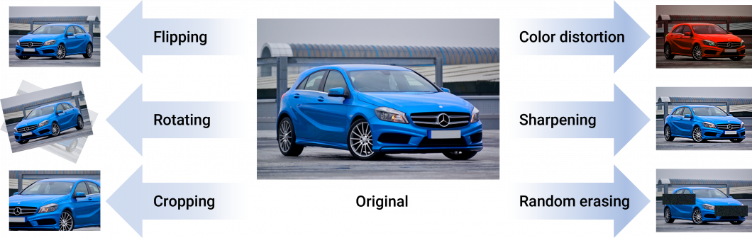
Data augmentation is a technique used to generate new training samples by applying various transformations to the original images. This process helps improve the model’s generalization capabilities by increasing the diversity of the training data, making the model more robust to variations in input data.
Common data augmentation techniques include rotation, scaling, flipping, and color jittering. All those techniques introduce variability without altering the underlying content of the images.
Handling Class Imbalance
Class imbalance can lead to biased model performance, where the model performs well on the majority class but poorly on the minority class. Addressing class imbalance is crucial for achieving accurate and reliable model performance.
Strategies for handling class imbalance include resampling, which involves oversampling the minority class, undersampling the majority class, or a combination of both. Synthetic data generation techniques, such as Synthetic Minority Over-sampling Technique (SMOTE), can also be employed.
Additionally, adjusting the model’s learning process, for example, through class weighting, can help mitigate the effects of class imbalance.
Benchmarking and Comparing Models
A thorough evaluation should involve benchmarking and performance measures for comparing different ML models:
Importance of benchmarking
Benchmarking is used to compare models because it provides a standardized and objective way to assess their performance, enabling developers to identify the most suitable model for a particular task or application.
By comparing models on common datasets and evaluation metrics, benchmarking facilitates informed decision-making and promotes continuous improvement in computer vision model development.
Popular public data sets for benchmarking
Popular public data sets for benchmarking computer vision models cover various tasks, such as image classification, object detection, and segmentation. Some widely-used data sets include:
- ImageNet: A large-scale dataset containing millions of labeled images across thousands of classes, primarily used for image classification and transfer learning tasks.
- COCO (Common Objects in Context): MS COCO is a popular dataset with diverse images featuring multiple objects per image, used for object detection, segmentation, and captioning tasks.
- Pascal VOC (Visual Object Classes): This important dataset contains images with annotated objects belonging to 20 classes, used for object classification and detection tasks.
- MNIST (Modified National Institute of Standards and Technology): A dataset of handwritten digits commonly used for image classification and benchmarking in machine learning.
- CIFAR-10/100 (Canadian Institute for Advanced Research): Two datasets consisting of 60,000 labeled images, divided into 10 or 100 classes, used for image classification tasks.
- ADE20K: A dataset with annotated images for scene parsing, which is used to train models for semantic segmentation tasks.
- Cityscapes: A dataset containing urban street scenes with pixel-level annotations, primarily used for semantic segmentation and object detection in autonomous driving applications.
- LFW (Labeled Faces in the Wild): A dataset of face images collected from the internet, used for face recognition and verification tasks.


Comparing performance metrics
Evaluating multiple models involves comparing their performance measures (e.g., Precision, Recall, F1 score, AUC) to determine which model best meets the specific requirements of a given application. It is important to consider the specific applications of your application.
Below is a table to guide you on how to compare metrics:
| Metric | Goal | Ideal Value | Importance |
|---|---|---|---|
| Precision | Correct positive predictions | High | Crucial when the cost of false positives is high or when minimizing false detections is desired. |
| Recall | Identify all positive instances | High | Essential when missing positive cases is costly or when detecting all positive instances is vital. |
| F1 Score | Balanced performance | High | Useful when dealing with imbalanced datasets or when false positives and false negatives have different costs. |
| AUC | Overall classification performance | High | Important for assessing the model’s performance across various classification thresholds and when comparing different models. |
Using multiple metrics for a comprehensive evaluation
Using multiple metrics for a comprehensive evaluation is crucial because different metrics capture various aspects of a model’s performance, and relying on a single metric may lead to a biased or incomplete understanding of the model’s effectiveness.
By considering multiple metrics, developers can make more informed decisions when selecting or tuning models for specific applications. For example:
- Imbalanced datasets: In cases where one class significantly outnumbers the other, accuracy can be misleading, as a high accuracy might be achieved by predominantly classifying instances into the majority class. In this scenario, using Precision, Recall, and F1 score can provide a more balanced assessment of the model’s performance, as they consider the distribution of both positive and negative predictions.
- Varying costs of errors: When the costs associated with false positives and false negatives are different, using a single metric like accuracy or precision might not be sufficient. In this case, the F1 score is useful, as it combines both Precision and Recall, providing a balanced measure of the model’s performance while considering the trade-offs between false positives and false negatives.
- Classification threshold: The choice of classification threshold can significantly impact the model’s performance. By analyzing metrics like the AUC (Area Under the Curve) and the Precision-Recall Curve, developers can understand how the model’s performance varies with different thresholds and choose an optimal threshold for their specific application.

Evaluate Regression Models
To assess the effectiveness of regression models, it is important to be familiar with a set of regression metrics. In the following, we will look into the most important regression metrics and models.
Types of Regression Models
- Linear Regression: Linear regression is one of the simplest regression models. It assumes a linear relationship between the input features and the target variable. The goal is to find the best-fitting linear equation that minimizes the sum of squared errors between predicted and actual values.
- Polynomial Regression: Polynomial regression extends linear regression by allowing for higher-order polynomial functions. It can capture more complex relationships between variables.
- Ridge Regression and Lasso Regression: These are regularization techniques applied to linear regression to prevent overfitting. Ridge adds L2 regularization, while Lasso adds L1 regularization to the linear regression cost function.
- Support Vector Regression (SVR): SVR is an extension of support vector machines for regression tasks. It aims to find a hyperplane that has a maximum margin from the data points, while still fitting the data as closely as possible.
- Decision Trees and Random Forests: Decision trees can be used for regression tasks by splitting data into branches based on feature values. Random Forests are ensembles of decision trees that can provide more robust regression models.
- Gradient Boosting Regressors: Algorithms like Gradient Boosting and XGBoost build regression models by combining the predictions of multiple weak learners (usually decision trees) in an iterative manner.
Important Regression Metrics
When evaluating regression models, it’s important to collect the most appropriate metric based on the specific problem and domain. Different metrics are useful to measure different aspects of model performance. Additionally, cross-validation and visualizations, such as residual plots, can help provide a more comprehensive understanding of model performance.
- Mean Absolute Error (MAE): MAE calculates the average absolute difference between predicted and actual values. It provides a straightforward measure of how far off your predictions are on average.
MAE = (1/n) * Σ | actual - predicted | - Mean Squared Error (MSE): MSE determines the average of the squared difference between predicted and actual values. Compared to MAE, MSE penalizes larger errors more through squaring.
MSE = (1/n) * Σ (actual - predicted) ^2 - Root Mean Squared Error (RMSE): RMSE is the square root of MSE, which gives the error in the same units as the target variable, making it more interpretable.
RMSE = sqrt(MSE) - R-squared (R2) Score: R-squared measures the proportion of the variance in the target variable that is explained by the model. The R2 Score ranges from 0 to 1, with higher values indicating a better fit.
R2 = 1 - ( MSE(model) / MSE(mean) ) - Adjusted R-squared: Adjusted R-squared accounts for the number of predictors in the model and provides a more accurate measure of model fit when multiple features are involved.
- Mean Absolute Percentage Error (MAPE): MAPE expresses the error as a percentage of the actual value and is useful when you want to understand the error relative to the magnitude of the target variable.
MAPE = (1/n) * Σ | (actual - predicted) / actual | * 100
A Brief Recap
In this article, we highlighted the significance of computer vision model performance evaluation, covering essential performance metrics, evaluation techniques, dataset factors, and benchmarking practices. Accurate and continuous evaluation is critical for advancing and refining computer vision models.
As a data scientist, understanding these evaluation methods is key to making informed decisions when selecting and optimizing models for your specific use case. By employing multiple performance metrics and taking dataset factors into account, you can ensure that your computer vision models achieve the desired performance levels and contribute to the progress of this transformative field. It is important to iterate and refine your models to attain the best possible results in your computer vision applications.