Data Science Tutorial using Python

Data science is a multidisciplinary field that relies on scientific methods, statistics, and Artificial Intelligence (AI) algorithms to extract knowledgeable and meaningful insights from data. At its core, data science is all about discovering useful patterns in data and presenting them to tell a story or make informed decisions.

About us: Viso.ai provides a robust end-to-end computer vision infrastructure – Viso Suite. Our software helps several leading organizations start with computer vision and implement deep learning models efficiently with minimal overhead for various downstream tasks.

Fundamentals of Data Engineering

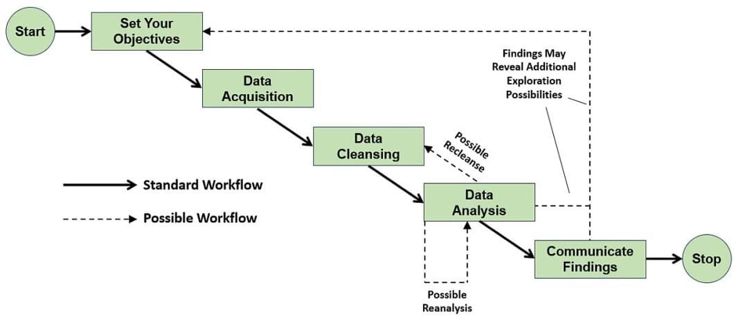
Data Acquisition

The first step in the data science process is to define the research goal. The next step is to acquire appropriate data that will enable you to derive insights. Data may come from relational databases, spreadsheets, inventories, external APIs, etc. During this stage, it is reasonable to check that the data is in the correct format for your purposes.

The types of data to acquire are tailored towards the type of problem you want to solve. Therefore, you need to identify appropriate datasets if they already exist, or most likely, create one ourselves. The data acquisition step may include sourcing data within the organization or leveraging external data sources.

Data Preparation

The preparation of data involves three main mini-steps. Data cleansing, data transformation, and data combination. Moreover, the data preparation step changes the raw real-world data. Then the scientists and analysts can analyze these data with a computer, i.e. a machine learning algorithm.

First, you clean the datasets you have obtained. You perform this by identifying missing values, errors, outliers, etc. Most machine learning algorithms cannot handle missing values, so replacing or removing them is advisable. Also, in this phase, we clean the outliers, i.e., data points far from the observed distribution.

Data transformation refers to aggregating data, dealing with categorical variables, and creating dummies to ensure consistency. Also, it reduces the number of variables and retains the most informative features. It discards the redundant features by scaling the data, etc.

Data Exploration

The data exploration stage observes the data closely to understand what it is about. This step involves using statistical metrics such as mean, median, mode, variance, etc. to describe the data distribution. Common data visualization techniques display the exploratory data by bar charts, pie charts, histograms, line graphs, etc.

By visualization, you can identify anomalies in your data and have a better representation of your data content. Anomalies in the exploratory data analysis are corrected by going back to the previous step, data preparation. In addition, data exploration enables you to discover patterns that you may combine with domain knowledge and create new informative features.

Data Modeling

In the data modeling step, you take a more involved approach when accessing the data. Data modeling involves choosing an algorithm, usually from the related fields of statistics, data mining, or machine learning models. It then involves deciding which features to include in the algorithm as the input, executing the model, and finally evaluating the trained model for performance.

You choose features that show the most variability across your data distribution. You drop features that do not drive the final prediction or are uninformative. Techniques such as Principal Component Analysis (PCA) can help to identify important features.

The next step involves choosing an appropriate algorithm for the learning task. Different algorithms are better suited to different learning problems. Logistic regression, Naive Bayes classifier, Support Vector Machines, decision trees, and random forests are some popular classification algorithms with good performance.

Linear regression and neural networks are practical for regression tasks. Various modeling algorithms exist, and scientists don’t know the best ones until they try them. Therefore, keeping an open mind and relying heavily on experimentation is important.

Python Data Science Tools and Libraries

Scikit-learn

Scikit-Learn is the most popular machine-learning library in the Python programming ecosystem. Skicit is a mature Python library and contains several algorithms for classification, regression, and clustering. Many common algorithms are available in Scikit-Learn and it exposes a consistent interface to access them.

Therefore, learning how to work with one classifier in Scikit-Learn means that you can work with other methods. Also, it possesses methods to train a classifier regardless of the underlying implementation.

You would rely heavily on Scikit-Learn for your modeling tasks as you dive deeper into data science. Here is a simple example of creating a classifier and training it on one of the bundled datasets.

#  sample  decision  tree  classifier from  sklearn  import  datasets
from  sklearn  import  metrics
from  sklearn.tree import  DecisionTreeClassifier
# load the iris datasets dataset = datasets.load_iris()
#  fit  a  CART  model  to  the  data model  =  DecisionTreeClassifier()
model.fit(dataset.data,  dataset.target) print(model)
# make predictions expected = dataset.target
predicted  =  model.predict(dataset.data)
#  summarize  the  fit  of  the  model print(metrics.classification_report(expected,  predicted)) print(metrics.confusion_matrix(expected,  predicted))

You can find more information about Scikit-Learn here.

NymPy – Numerical Python

NumPy is the main numerical computing library for Python programming language. It provides access to a multidimensional array object and exposes several methods that use operations over arrays. It supports linear algebra operations such as matrix multiplication, inner product, identity operations, etc.

NumPy interfaces with low-level libraries written in C and Fortran thereby producing faster and more efficient outputs. As a result, Python control structures like loops are not present in performing numerical computation (they are significantly slower).

NumPy can be seen as a set of Python APIs that enables efficient scientific computing. E.g., NumPy arrays can be initiated by nested Python lists. The level of nesting specifies the rank of the array.

import  numpy  as  np
a = np.array([[1, 2, 3], [4, 5, 6]])   # creates a rank 2 array print(type(a))
print(a.shape)

The array created is of rank 2 which means that it is a matrix. We can see this clearly from the size of the array printed. It contains 2 rows and 3 columns hence size (m, n).

You can find more information about NumPy here.

ScyPy – Scientific Python

SciPy is a scientific computing library geared toward the fields of mathematics, science, and engineering. It functions together with NumPy and extends it by providing additional modules for optimization, technical computing, statistics, signal processing, etc.

Data science engineers utilize SciPy mostly in conjunction with other tools in the ecosystem, like Pandas and Matplotlib. Here is a simple usage of SciPy that finds the inverse of a matrix.

from  scipy  import  linalg
z = np.array([[1,2],[3,4]]) print(linalg.inv(z))</code>

[ [-2.  1.]
[1.5  -0.5 ] ]

Matplotlib

Matplotlib is a plotting library that integrates nicely with NumPy and other numerical computation libraries in Python. Thus, it is capable of producing quality plots and charts. Data scientists widely use it in data exploration where visualization techniques are important.

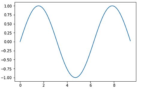
Matplotlib exposes an object-oriented API making it easy to create powerful visualizations in Python. Note that to see the plot in Jupyter Notebooks you must use the Matplotlib inline magic command. Here is an example that uses Matplotlib to plot a sine waveform.

import  matplotlib.pyplot  as  plt
#  compute  the  x  and  y  coordinates  for  points  on  a  sine  curve x = np.arange(0, 3 * np.pi, 0.1)
y = np.sin(x)
#  plot  the  points  using  matplotlib plt.plot(x, y)
plt.show()   #  Show  plot  by  calling  plt.show()

You can find more information about Matplotlib here.

Pandas

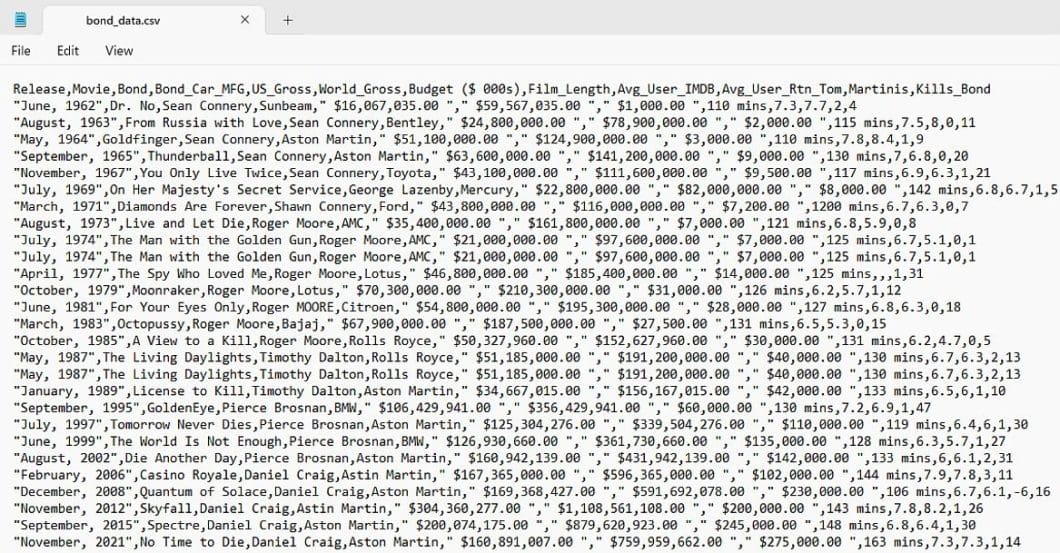
Pandas is a data manipulation library in Python that offers high-performance data structures for time series data. Data engineers utilize Pandas extensively for data analysis and most data loading, cleaning, and transformation tasks. Data from the real world is usually messy, contains missing values, and needs transformation.

Pandas accept data file types like CSV, Excel spreadsheets, Python pickle format, JSON, SQL, etc. There exist two main types of Pandas data structures, series and data frame. Series is the data structure for a single data column, while a data frame stores 2-dimensional data, i.e. matrix. Subsequently, a data frame contains data stored in many columns.

The code below shows how to create a Series object in Pandas.

import  pandas  as  pd
s = pd.Series([1,3,5,np.nan,6,8]) print(s)

To create a data frame, you can run the following code.

df  =  pd.DataFrame(np.random.randn(6,4),  columns=list('ABCD')) print(df)

Pandas loads the file formats it supports into a data frame and manipulation of the data frame occurs using Pandas methods.

Implementing Data Science Algorithms in Python

Binary and Multiclass Classification

A common machine learning task is to classify a data variable into two or more categories. In binary classification, the scientists categorize the dataset into two classes. Consequently, they categorize data into several classes based on the classification rules in multi-class classification.

The Python code for the binary classification and its visualization is as below.

from mlxtend. evaluate import confusion_matrix
y_target =    [0, 0, 1, 0, 0, 1, 1, 1]
y_predicted = [1, 0, 1, 0, 0, 0, 0, 1]
cm = confusion_matrix(y_target=y_target, y_predicted=y_predicted)
import matplotlib.pyplot as plt
from mlxtend.plotting import plot_confusion_matrix
fig, ax = plot_confusion_matrix(conf_mat=cm)
plt.show()

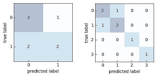
The Python code for the multi-class classification and its visualization is as below.

from mlxtend.evaluate import confusion_matrix
y_target =    [1, 1, 1, 0, 0, 2, 0, 3]
y_predicted = [1, 0, 1, 0, 0, 2, 1, 3]
cm = confusion_matrix(y_target=y_target, y_predicted=y_predicted, binary=False)
import matplotlib.pyplot as plt
from mlxtend.evaluate import confusion_matrix
fig, ax = plot_confusion_matrix(conf_mat=cm)
plt.show()

Decision Trees Implementation

A decision tree is a machine learning algorithm that is mainly used for classification that constructs a tree of possibilities. The branches in the tree represent decisions and the leaves represent label classification.

The purpose of a decision tree is to create a structure where samples in each branch are homogenous or of the same type. It does this by splitting samples in the training data according to specific attributes that increase homogeneity in branches. Therefore, the attributes form the decision node along which samples are separated.

We will present an example using Python, Scikit-Learn, and decision trees. We would tackle a multi-class classification problem where the challenge is to classify wine into three types using features such as alcohol, color intensity, hue, etc. The data we would use is from the wine recognition dataset by UC Irvine. You can find the dataset and the accompanying code here.

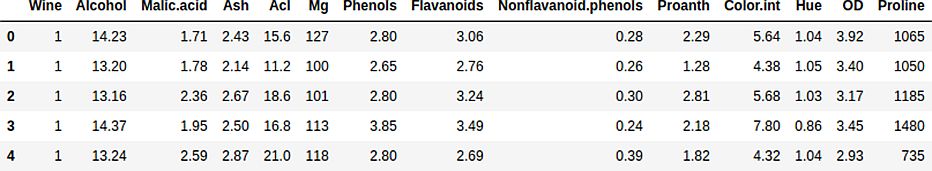
First, we’ll load the dataset and use the Pandas head method to take a look at it.

import  numpy  as  np import  pandas  as  pd
import  matplotlib.pyplot  as  plt
%matplotlib  inline
dataset  =  pd.read_csv('wine.csv')
dataset.head(5)
features  =  dataset.drop(['Wine'],  axis=1) labels  =  dataset['Wine']

To evaluate our model well, we divide the dataset into a train and test split. Then, the last step is to import the decision tree classifier and fit it to our data.

from  sklearn.model_selection  import  train_test_split
features_train, features_test,  labels_train,     labels_test=     train_test_split(features, labels, test_size=0.25)
from  sklearn.tree  import  DecisionTreeClassifier classifier  =  DecisionTreeClassifier()
classifier.fit(features_train,  labels_train)

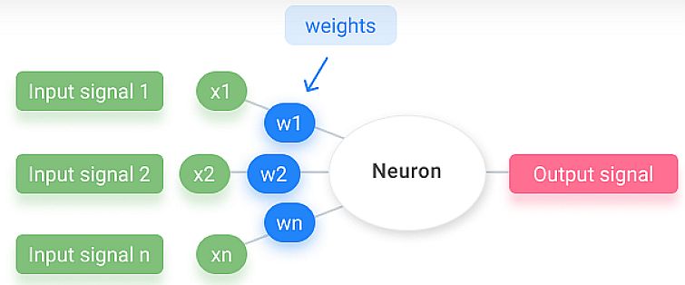
Neural Network Implementation

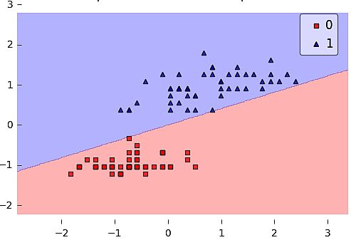
The neural network receives multiple input signals, and if the sum of the input signals exceeds a given threshold, it activates a signal or stays calm otherwise. The algorithm learns the weights for the input signals to deduct the decision value, which allows you to differentiate between the two separate classes +1 and -1.

The following example is about iris flowers classification into two categories (class 1 and class 2). When we run the code – the perceptron iterates 5 times. The bias and weights are: [[-0.04500809] [ 0.11048855]].

from mlxtend.data import iris_data
from mlxtend.plotting import plot_decision_regions
from mlxtend.classifier import Perceptron
import matplotlib.pyplot as plt
# Loading Data
X, y = iris_data()
X = X[:, [0, 3]] # sepal length and petal width
X = X[0:100] # class 0 and class 1
y = y[0:100] # class 0 and class 1
# standardize
X[:,0] = (X[:,0] - X[:,0].mean()) / X[:,0].std()
X[:,1] = (X[:,1] - X[:,1].mean()) / X[:,1].std()
# Rosenblatt Perceptron
ppn = Perceptron(epochs=5, eta=0.05, random_seed=0, print_progress=3)
ppn.fit(X, y)
plot_decision_regions(X, y, clf=ppn)
plt.title('Perceptron Rule')
plt.show()
print('Bias & Weights: %s' % ppn.w_)
plt.plot(range(len(ppn.cost_)), ppn.cost_)
plt.xlabel('Iterations')
plt.ylabel('Missclassifications')
plt.show()

Implementing Data Analytics

That was a quite concise Python data science tutorial. Data science in Python allows you to monitor your data in real-time. You can bring the data from your deployed AI or machine learning applications of data together in cloud dashboards.

If you want to learn data science and explore similar topics, check out our other blogs:

• Data Preprocessing Techniques for Machine Learning with Python
• Complete Guide to Feature Extraction in Python
• A Straightforward Tutorial of Streamlit
• Getting Started With Kaggle: A Comprehensive Guide
• Concept Drift vs Data Drift: How AI Can Beat the Change
• Online Computer Vision and Python Courses: How to Start with Data Science

Data Management with Viso Suite

While Viso Suite infrastructure provides teams with full control over the application lifecycle, let’s discuss how it leverages data analytics for business. A key benefit of the computer vision infrastructure is the ability to evolve and scale with the needs of the business. We have several features supporting this:

• Real-time Insights: made possible by processing real-time visual data at the edge. This gives companies a competitive advantage in applications security monitoring, quality control in manufacturing, and customer behavior analysis in retail.
• Predictive Analytics: through reading historical data to forecast future behavior and outcomes. This enables strategic planning and proactive measures in business.
• Enhanced Decision-making: with customized dashboards, data visualization, and feedback. Businesses can make data-informed decisions and not worry that their data provides an incomplete picture of the use cases at hand.
• Operational Efficiency: by identifying bottlenecks and inefficiencies in business processes. This could look like identifying gaps in logistics processes that slow down the transport of goods from warehouses to shipping facilities to final destinations.

With Viso Suite, our team of experts supports businesses in the development, implementation, management, and securing of large-scale computer vision systems. Our industry-agnostic infrastructure makes it possible for teams around the world to solve business challenges and optimize workflows with computer vision. To learn more about how Viso Suite can elevate your use case, reach out to our team by clicking the “get started” button below.