
Feature Extraction is the process of transforming raw data, often unorganized, into meaningful features. These are then used to train machine learning models. In today’s digital world, machine learning algorithms are used widely for credit risk prediction, stock market forecasting, early disease detection, etc. The accuracy and performance of these models rely on the quality of the input features. In this blog, we will introduce you to feature engineering, why we need it, and the different machine learning techniques available to execute it.
What is Feature Extraction in Machine Learning?
We provide training data to machine learning models to help the algorithm learn underlying patterns to predict the target/output. The input training data is referred to as ‘features’, vectors representing the data’s characteristics. For example, let’s say the objective is to build a model to predict the sales of all air conditioners on an e-commerce site. What data will be useful in this case? It would help to know the product features like its power-saving mode, rating, warranty period, installation service, seasons in the region, etc. Among the sea of information available, selecting only the significant and essential features for input is called feature extraction.
The type of features and extraction techniques also vary depending on the input data type. While working with tabular data, we have both numerical (e.g. Age, No of products, and categorical features (Gender, Country, etc). In deep learning models that use image data, features include detected edges, pixel data, exposure, etc. In NLP models based on text datasets, features can be the frequency of specific terms, sentence similarity, etc.
What is the Difference Between Feature Extraction and Feature Learning?
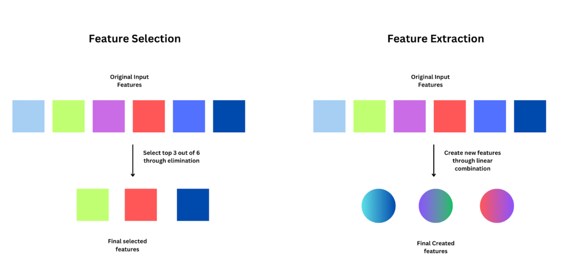
Beginners often get confused between feature selection and feature extraction. Feature selection is simply choosing the best ‘K’ features from available ‘n’ variables, and eliminating the rest. Whereas feature extraction involves creating new features through combinations of the existing features.
Before we dive into the various methods for feature extraction, you need to understand why we need it, and the benefits it can bring.
Why do we Need Feature Extraction?
In any data science pipeline, feature extraction is done after data collection and cleaning. One of the simplest but accurate rules in machine learning: Garbage IN = Garbage OUT! Let’s take a look at why feature engineering is needed and how it benefits building a more efficient and accurate model.
- Avoid Noise & Redundant Information: Raw data can have a lot of noise due to gaps and manual errors in data collection. You may also have multiple variables that provide the same information, becoming redundant. For example, if both height and weight are included as features, including their product (BMI) will make one of the original features redundant. Redundant variables do not add additional value to the model; instead may cause overfitting. Feature extraction helps in removing noise and redundancy to create a robust model with extracted features.
- Dimensionality Reduction: Dimensionality refers to the number of input features in your machine-learning model. High dimensionality may lead to overfitting and increased computation costs. Feature extraction provides us with techniques to transform the data into a lower-dimensional space while retaining the essential information by reducing the number of features.
- Improved & Faster Model Performance: Feature extraction techniques help you create relevant and informative features that provide variability to the model. By optimizing the feature set, we can speed up model training and prediction processes. This is especially helpful when the model is running in real-time and needs scalability to handle fluctuating data volumes.
- Better Model Explainability: Simplifying the feature space and focusing on relevant patterns improves the overall explainability (or interpretability) of the model. Interpretability is crucial to know which factors influenced the model’s decision, to ensure there is no bias. Improved explainability makes it easier to justify compliance with data privacy regulations in financial and healthcare models.
With a reduced set of features, data visualization methods are more effective in capturing trends between features and output. Apart from these, feature extraction allows domain-specific knowledge and insights to be incorporated into the modeling process. While creating features, you should also take the help of domain experts.
Principal Component Analysis (PCA) for Feature Extraction
PCA or Principal Component Analysis is one of the widely used methods to battle the “curse of dimensionality”. Let’s say we have 200 features in a dataset, will all of them have the same impact on the model prediction? No. Different subsets of features have different variances in the model output. PCA aims to reduce the dimension while also maintaining model performance, by retaining features that provide maximum variance.
How Does PCA Work?
The first step in PCA is to standardize the data. Next, it computes a covariance matrix that shows how each variable interacts with other variables in the dataset. From the covariance matrix,
PCA selects the directions of maximum variance, also called “principal components,” through Eigenvalue decomposition. These components transform the high-dimensional data into a lower-dimensional space.
How to Implement PCA Using Scikit-Learn?
I’ll be using a weather dataset to predict the probability of rain as an example to show how to implement PCA. You can download the dataset from Kaggle. This dataset contains about 10 years of daily weather observations from many locations across Australia. Rain Tomorrow is the target variable to predict.
Step 1: Start by importing the essential packages as part of the preprocessing steps.
# Import necessary packages
import numpy as np
import pandas as pd
import seaborn as sb
import matplotlib.pyplot as plt
from sklearn import preprocessing # To get MinMax Scaler function
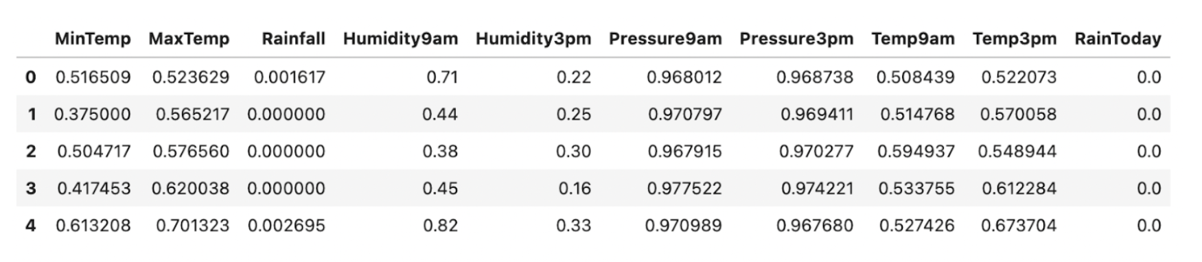
Step 2: Next, read the CSV file into a data frame and split it into Features and Target. We are using the Min Max scaler function from sklearn to standardize the data uniformly.
# Read the CSV file
data = pd.read_csv('../input/weatherAUS.csv')


# Split the target var (Y) and the features (X)
Y = data.RainTomorrow
X = data.drop(['RainTomorrow'], axis=1)


# Scaling the dataset
min_max_scaler = preprocessing.MinMaxScaler()
X_scaled = pd.DataFrame(min_max_scaler.fit_transform(X), columns = X.columns)
X_scaled.head()
Step 3: Initialize the PCA class from sklearn.decomposition module. You can pass the scaled features to ‘pca.fit()’ function as shown below.
# Initializing PCA and fitting

from sklearn.decomposition import PCA

pca = PCA()

pca.fit(X_scaled)
PCA will then compute the variance for different principal components. The ‘pca.explained_variance_ratio_’ captures this information. Let’s plot this to visualize how variance differs across feature space.
plt.plot(pca.explained_variance_ratio_, linewidth=2)

plt.axis('tight')

plt.xlabel('Number of Feautres')

plt.ylabel('Variance Ratio')
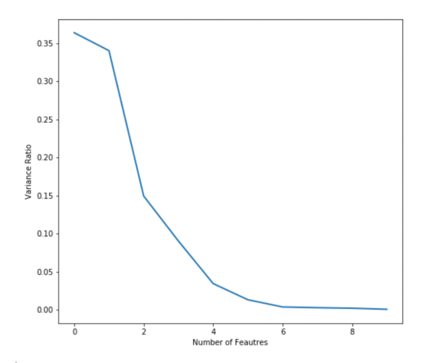
From the plot, you can see that the top 3-4 features can capture maximum variance. The curve is almost flat beyond 5 features. You can this plot to decide how many final features you want to extract from PCA. I’m choosing 3 in this case.
Step 4: Now, initialize PCA again by providing the parameter ‘n_components’ as 3. This parameter denotes the number of principal components or dimensions that you’d like to reduce the feature space to.
pca = PCA(n_components=3)

pca.fit_transform(x_train)
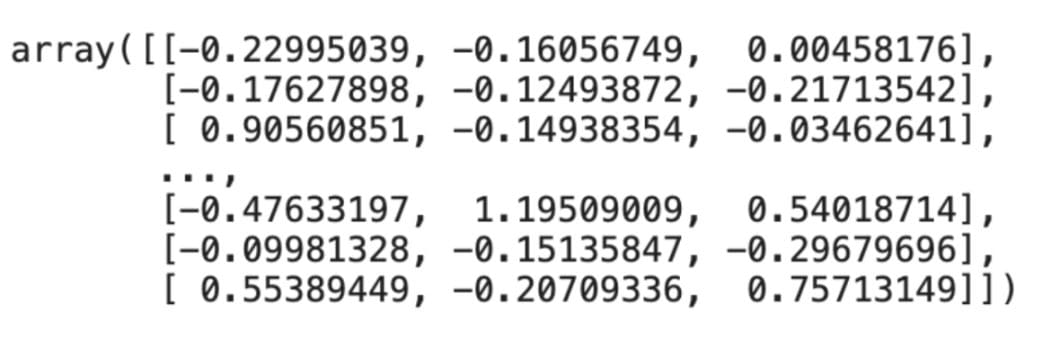
We have reduced our dataset to 3 features as shown above. If you want to check the total variance captured by the chosen components, you can calculate the sum of the explained variance.
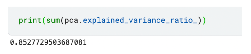
The reduced set of 3 features captures 85% variance amongst all features!
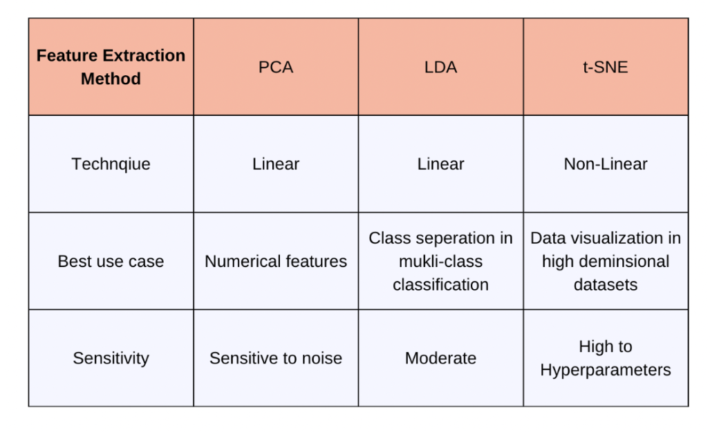
It’s best to use PCA when the number of features is too huge to visualize or interpret clearly. PCA can also handle multilaterally, but it is sensitive to outliers present. Ensure clean data by removing outliers, scaling, and standardizing.
LDA for Feature Extraction
Linear Discriminant Analysis (LDA) is a statistical technique widely used for dimensionality reduction in classification problems. The aim is to find a set of linear combinations of features that best separate the classes in the data.
How is LDA Different from PCA?
PCA targets only maximizing data variance, which is best in regression problems. LDA targets to maximize the differences between classes, which is ideal for multi-classification problems.
Let’s take a quick look at how LDA works:
- LDA requires the input data to be normally distributed and computes covariance matrices
- Next, LDA calculates two types of scatter matrices:
- Between-class scatter matrix: It is computed to measure the spread between different classes.
- Within-class scatter matrix: It computes the spread within each class.
- Eigenvalue Decomposition: LDA then performs eigenvalue decomposition on the matrix to obtain its eigenvectors and eigenvalues.
- The eigenvectors corresponding to the largest eigenvalues are chosen. These eigenvectors are the directions in the feature space that maximize class separability. We project the original data across these directions to obtain the reduced feature space.
How to Implement LDA on Classification Tasks?
Let’s create some synthetic data to play with. You can use the ‘make_classification()’ function from scikit-learn for this. Refer to the code snippet below. Once we create the data, we visualize it with a 3D plot.
from sklearn.datasets import make_classification

features, output = make_classification(

   n_features=10,

   n_classes=4,

   n_samples=1500,

   n_informative=2,

   random_state=5,

   n_clusters_per_class=1,

)

# Plot the 3D visualization

fig = px.scatter_3d(x=X[:, 0], y=X[:, 1], z=X[:, 2], color=y, opacity=0.8)

fig.show()
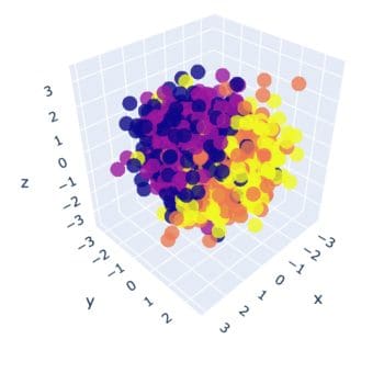
In the visualization, we can see 4 different colors for each class. It seems impossible to find any patterns currently. Next, import the LDA module from discriminant_analysis of scikit learn. Similar to PCA, you need to provide how many reduced features you want through the ‘n_components’ parameter.
From sklearn.discriminant_analysis import LinearDiscriminantAnalysis

# Initialize LDA

lda = LinearDiscriminantAnalysis(n_components=3)

post_lda_features = lda.fit(features, output).transform(features)

print("number of features(original):", X.shape[1])

print("number of features that was reduced:", post_flda_features.shape[1])
OUTPUT:

>> number of features(original): 10

>> number of features that was reduced: 3
We have successfully reduced the feature space to 3. You can also check the variance captured by each feature using the below command:
lda.explained_variance_ratio_

Now, let’s visualize the reduced feature space using the below script:
fig = px.scatter(x=post_lda_features[:, 0], y=post_lda_features[:, 1], color=y)
fig.update_layout(
   title="After LDA on feature space",
)
fig.show()
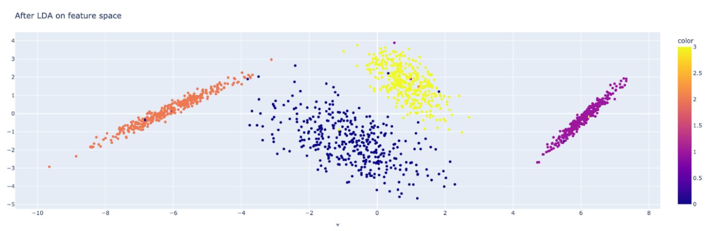
You can clearly see how LDA helped in separating the classes! Feel free to experiment with a different number of features, components, etc.
Feature Extraction with t-SNE
t-SNE stands for t-distributed Stochastic Neighbor Embedding. It is a non-linear technique preferred for visualizing high-dimensional data. This method aims to preserve the relationship between data points while reducing the feature space.
How does the Algorithm Work?
First, we represent each point in the dataset by a feature vector. Next, t-SNE calculates 2 probability distributions for each pair of data points:
- The first distribution represents the similarities between data points in the high-dimensional space
- The second distribution represents the similarities in the low-dimensional space
The algorithm then minimizes the difference between the two distributions, using a cost function. Mapping to lower dimensions: Finally, it maps the data points to the lower-dimensional space while preserving the local relationships.
Here’s a code snippet to quickly implement t-SNE using scikit-learn.
from sklearn.manifold import TSNE

tsne = TSNE(n_components=3, random_state=42)

X_tsne = tsne.fit_transform(X)

tsne.kl_divergence_
Let’s quickly plot the feature space reduced by t-SNE.
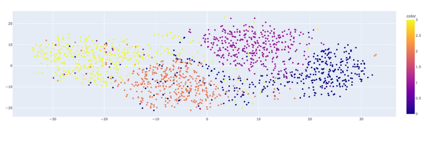
You can see the clusters for different classes of the original dataset and their distribution. As it preserves local relationships, it is the best method for visualizing clusters and patterns.
Specialized Feature Extraction Techniques
The methods discussed above are for tabular data. While dealing with text or image data, we have specialized feature extraction techniques. I’ll briefly go over some popular methods:
- Feature Extraction in Natural Language Processing (NLP): NLP models are built on large corpora of text data. Bag-of-Words (BoW) is a technique that represents text data by counting the frequency of each word in a document. Term Frequency-Inverse Document Frequency (TF-IDF) is also used. Techniques like Latent Dirichlet Allocation (LDA) or Non-Negative Matrix Factorization (NMF) are useful for extracting topics. They are useful in NLP tasks like document clustering, summarization, and content recommendation.
- Feature Extraction in Computer Vision: In computer vision, tasks like image processing, classification, and object detection are very popular. The Histogram of Oriented Gradients (HOG) computes histograms of gradient orientation in localized portions of an image. Feature Pyramid Networks (FPN) can combine features at different resolutions. Scale-Invariant Feature Transform (SIFT) can detect local features in images, robust to changes in scale, rotation, and illumination.
Implementing Feature Extraction with Python
Feature extraction is a crucial part of preparing quality input data and optimizing resources. We can also reuse pre-trained feature extractors or representations in related tasks, saving huge expenses. I hope you had a good read on the different techniques available in Python. When deciding which method to use, consider the specific goals of your analysis and the nature of your data. To reduce dimensionality while retaining as much variance as possible, PCA is a good choice. If your objective is to maximize class separability for classification tasks, LDA may be more appropriate. For visualizing complex numerical datasets and uncovering local structures, t-SNE is the go-to choice.
To learn more about computer vision, check out some of our other articles: