A Spatial Transformer Network (STN) is an effective method to achieve spatial invariance of a computer vision system. Max Jaderberg et al. first proposed the concept in a 2015 paper by the same name.
Spatial invariance is the ability of a system to recognize the same object, regardless of any spatial transformations. For example, it can identify the same car regardless of how you translate, scale, rotate, or crop its image. It even extends to various non-rigid transformations, such as elastic deformations, bending, shearing, or other distortions.
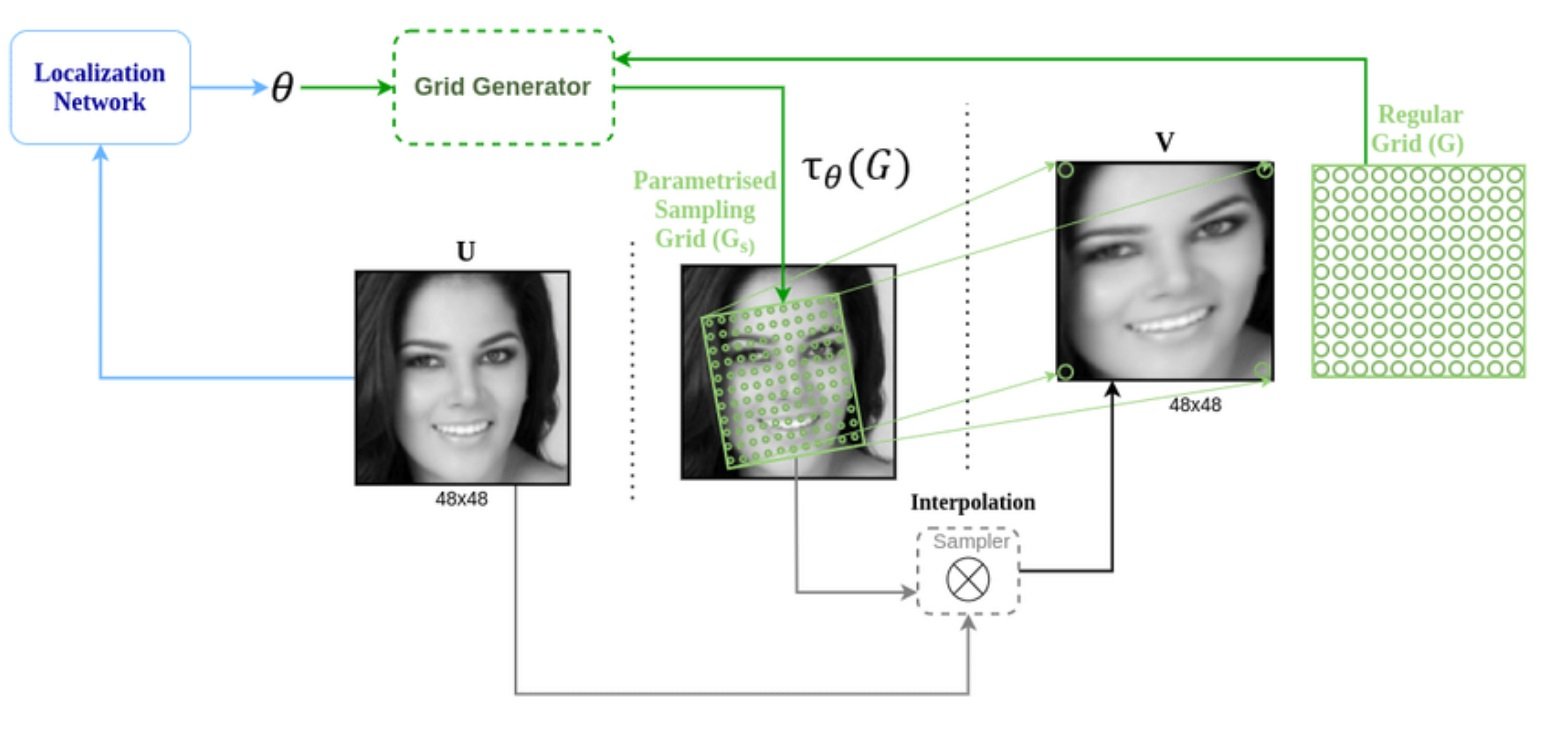
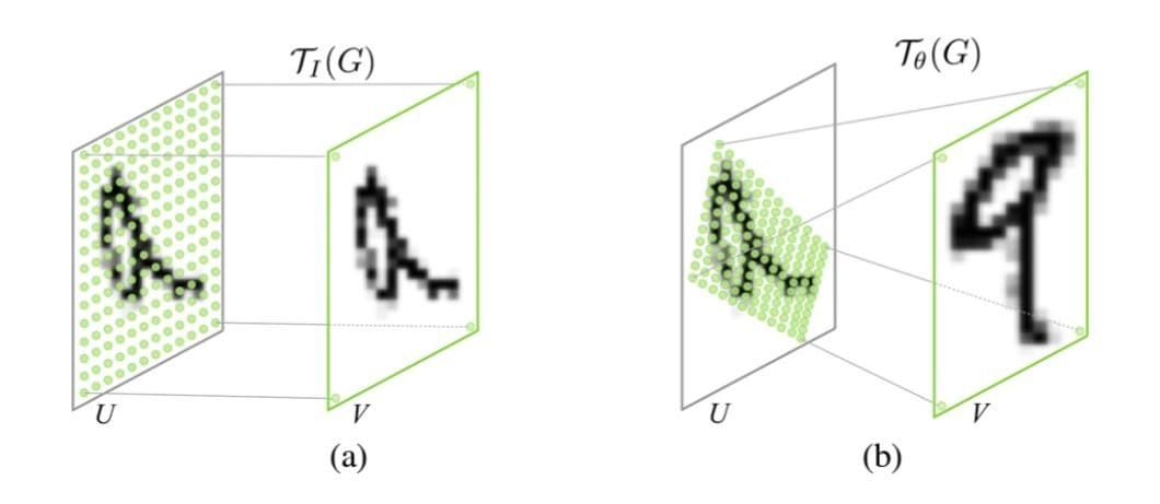
We’ll go into more detail regarding how exactly STNs work later on. However, they use what’s called “adaptive transformation” to produce a canonical, standardized pose for a sample input object. Going forward, it transforms each new instance of the object to the same pose. With instances of the object posed similarly, it’s easier to compare them for any similarities or differences.
STNs are used to “teach” neural networks how to perform spatial transformations on input data to improve spatial invariance.
In this article, we’ll delve into the mechanics of STNs, how to integrate them into the existing Convolutional Neural Network (CNN), and cover real-world examples and case studies of STNs in action.
Spatial Transformer Networks Explained
The central component of the STN is the spatial transformer module. In turn, this module consists of three sub-components: the localization network, the grid generator, and the sampler.
Spatial Transformer Module
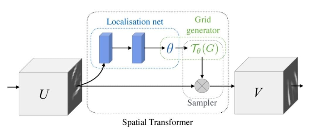
The idea of the separation of concerns is vital to how an STN works, with each component serving a distinct function. The interplay of components not only improves the accuracy of the STN but also its efficiency. Let’s look at each of them in more detail.
- Localization Network: Its role is to calculate the parameters that will transform the input feature map into the canonical pose, often through an affine transformation matrix. Typically, a regression layer within a fully-connected or convolutional network produces these transformation parameters.
The number of dimensions needed depends on the complexity of the transformation. A simple translation, for example, may only require 2 dimensions. A more complex affine transformation may require up to 6. - Grid Generator: Using the inverse of the transformation parameters produced by the localization net, the grid generator applies reverse mapping to extrapolate a sampling grid for the input image. Simply put, it maps the non-integer sample positions back to the original input grid. This way, it determines where in the input image to sample from to produce the output image.
- Sampler: Receives a set of coordinates from the grid generator in the form of the sampling grid. Using bilinear interpolation, it then extracts the corresponding pixel values from the input map. This process consists of three operations:
- Find the four points on the source map surrounding the corresponding point.
- Calculate the weight of each neighboring point based on proximity to the point.
- Produce the output by mapping the output point based on the results.
Other Features
The separation of responsibilities allows for efficient backpropagation and reduces computational overhead. In some ways, it’s similar to other approaches, like max pooling.
It also makes it possible to calculate multiple target pixels concurrently, speeding up the process through parallel processing.
STNs also provide an elegant solution to multi-channel inputs, such as RGB color images. It goes through an identical mapping process for each channel. This preserves spatial consistency across the different channels so that it doesn’t negatively impact accuracy.
Integrating STNs with CNNS has been shown to significantly improve spatial invariance. Traditional CNNs excel at hierarchically extracting features through convolution and max pooling layers. The introduction of STNs allows them to also effectively handle objects with variations in regards to orientation, scale, position, etc.
One poignant example is that of MNIST – a classic dataset of handwritten digits. In this use case, one can use an STN to center and normalize digits, regardless of input presentation. This makes it easier to accurately compare handwritten digits with many potential variations, dramatically lowering error rates.
Commonly Used Technologies and Frameworks For Spatial Transformer Networks
When it comes to implementation, the usual suspects, TensorFlow and PyTorch, are the go-to backbone for STNs. These deep learning frameworks come with all the necessary tools and libraries for building and training complex neural network architectures.
TensorFlow is well-known for its versatility in designing custom layers. This flexibility is key to implementing the various components of the spatial transformation module: the localization net, grid generator, and sampler.
On the other hand, PyTorch’s dynamic computational graphs make coding the otherwise complex transformation and sampling processes more intuitive. It’s built-in Spatial Transformer Networks support features the affine_grid and grid_sample functions to perform transformation and sampling operations.
Although STNs have inherently efficient architectures, some optimization is needed due to the complex use cases they handle. This is especially true when it comes to training these models.
Best practices include the careful selection of appropriate loss functions and regularization techniques. Both transformation consistency Loss and task-specific loss functions are typically combined to avoid STN transformations distorting the data and to ensure that the output data is useful for the task at hand, respectively.
Regularization techniques help avoid the issue of overfitting the model to its training data. This would negatively impact its ability to generalize for new or unseen use cases.
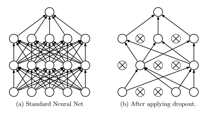
Several regularization techniques are useful in the development of STNs. These include dropout, L2 Regularization (weight decay), and early stopping. Of course, improving the size, scope, and diversity of the training data itself is also crucial.
Performance of Spatial Transformer Networks vs Other Solutions
Since its introduction in 2015, STNs have tremendously advanced the field of computer vision. They empower neural networks to perform spatial transformations to standardize variable input data.
In this way, STNs are helping to solve a stubborn weakness of most standard convolutional networks. I.e., the robustness to accurately execute computer vision tasks on datasets where objects have varying presentations.
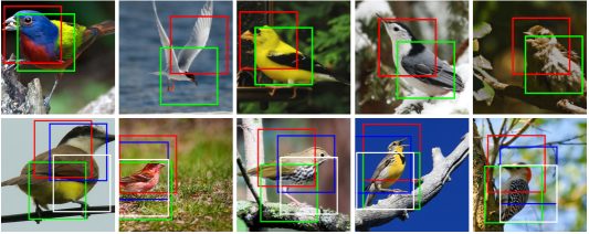
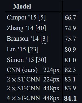
In the original paper, Jaderberg and co. tested the STN against traditional solutions using a variety of data. In noisy environments, the various models achieved the following error rates when processing MNIST datasets:
- Fully Convolutional Network (FCN): 13.2%
- CNN: 3.5%
- ST-FCN: 2.0%
- ST-CNN: 1.7%
As you can see, both the spatial transformer-containing models significantly outperformed their conventional predecessors. In particular, the ST-FCN outperformed the standard FCN by a factor of 6.
Further Research
Other research has shown promising results integrating STNs with other models, like Recurrent Neural Networks (RNNs). In particular, this marriage has shown substantial performance improvements in sequence prediction tasks. This involves, for example, digit recognition on cluttered backgrounds, similar to the MNIST experiment.
The paper’s proposed RNN-SPN model achieved an error rate of just 1.5% compared to 2.9% for a CNN and 2.0% for a CNN with SPN layers.
Generative Adversarial Networks (GANs) are another type of model with the potential to benefit from STNs, as so-called ST-GANs. STNs may very well help to improve the sequence prediction as well as image generation capabilities of GANs.
Real-World Applications and Case Studies of Spatial Transformer Networks
The wholesale benefits of STNs and their versatility mean they are being used in a wide variety of use cases. STNs have already proven their potential worth in several real-world situations:
- Healthcare: STNs are used to heighten the precision of medical imaging and diagnostic tools. Subjects such as tumors may have highly nuanced differences in appearance. Apart from actual medical care, they can also be used to improve compliance and operational efficiency in hospital settings
- Autonomous Vehicles: Self-driving and driver-assist systems have to deal with dynamic and visually complex scenarios. They also need to be able to perform in real-time to be useful. STNs can aid in both by improving trajectory prediction, thanks to their relative computational efficiency. Performance in these scenarios can be further improved by including temporal processing capabilities.

- Robotics: In various robotics applications, STNs contribute to more precise object tracking and interaction. This is especially true for complex and new environments where the robot will perform object-handling tasks.
In a telling case study, researchers proposed TransMOT, a Spatial-Temporal Graph Transformer for Multiple Object Tracking. The goal of this study was to improve the ability of robotics systems to handle and interact with objects in varied environments. The team implemented STNs, specifically to aid the robot’s perception systems for improved object recognition and manipulation.
Indeed, variations and iterations of the TransMOT model showed significant performance increases over its counterparts in a range of tests.
What’s Next for Spatial Transformer Networks?
To continue learning about machine learning and computer vision, check out our other blogs:
