
Neural Networks have changed the way we perform model training. Present day, we see many neural network varieties applied across the field of machine learning: Convolutional Neural Networks, Recurrent Neural Networks, Liquid Neural Networks, and more. These advancements have paved the way for the emergence of a subset of machine learning: Deep Learning.
With the increase in the usage of computers and machine learning systems, the availability of data has become easy. Neural networks, sometimes referred to as Neural Nets, need large datasets for efficient training. This availability of data made it easy to train and adopt across the industry.
Even though they work efficiently, they do have some challenges. For example, if the model we trained encounters something outside the training set, it won’t work properly as it has never encountered it. Also, with large amounts of data, the complexity of the model increases. So, what if we have a neural network that can adapt itself to new data and has less complexity? Let’s dive in.
What is a Liquid Neural Network?
In the year 2020, researchers at MIT’s Computer Science and Artificial Intelligence Laboratory (CSAIL), Ramin Hasani, Daniela Rus, and the team introduced a kind of neural network known as Liquid Neural Networks (LNNs). LNNs are a type of Recurrent Neural Network (RNN) that is time-continuous.
Their dynamic architecture can adapt its structure based on the data. This is something similar to liquids that can take the shape of the container they are in. Hence, they are called Liquid Neural Networks. They can learn on the job even after training.
These neural networks are inspired by the nervous system of a microscopic worm known as C. elegans. It has 302 neurons. However, despite a low number of neurons, it can exhibit intricate behaviors which is too much for the number of neurons it has. Next, let’s see how these liquid neural networks work.
How do Liquid Neural Networks Work?
Liquid Neural Networks are a class of Recurrent Neural Networks (RNNs) that are time-continuous. LNNs are made up of first-order dynamical systems controlled by non-linear interlinked gates. The end model is a dynamic system with varying time constants in a hidden state. This is an improvement of Recurrent Neural Networks where time-dependent independent states are introduced.
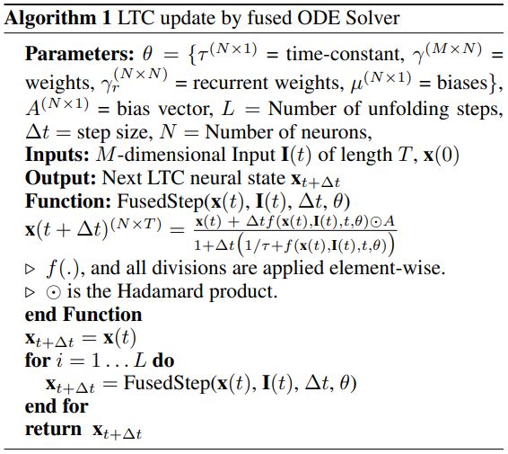
Numerical differential equation solvers compute the outputs. Each differential equation represents a node of that system. The closed-form solution makes sure that they perform well with a smaller number of neurons. This gives rise to fewer and richer nodes.
They show stable and bounded behavior with improved performance on time series data. The differential equation solver updates the algorithm as per the below-given rules.
LNN architecture has three layers. They are:
- Input layer.
- Liquid layer (Reservoir).
- Output layer.
Input layer: This is the layer that has the inputs to the network. All the input data that we want to train the model on is given to this layer. This layer feeds the input data to the liquid layer.
Liquid layer: This layer is also known as a reservoir. It contains a large recurrent network of neurons. They are initialized with synaptic weights. Input data is transformed into a rich non-linear space.
Output layer: It consists of output neurons. This receives the information from the liquid layer.
Now, let’s see how to implement a simple Liquid Neural Network using TensorFlow.
Implementation of a Liquid Neural Network (LNN)
We will use the MNIST dataset available in the TensorFlow datasets. MNIST dataset contains handwritten digits and is widely used for educational and research purposes. It has 70000 samples, of which 60000 samples are used as a training dataset, and the rest of the samples are used as a test dataset. The dimension of each image is (28,28,1).
Import Libraries
To implement LNN, we will begin by importing the necessary libraries as shown below:
import numpy as np
import tensorflow as tf
from tensorflow import keras
In the code above, we have imported Numpy, TensorFlow, and Keras.
Define Weight Initialize, Train, and Predict Functions
Next, we define a function to initialize the weights of the model.
def initialize_weights(input_dim, reservoir_dim, output_dim, spectral_radius):
    # Initialize reservoir weights randomly
    reservoir_weights = np.random.randn(reservoir_dim, reservoir_dim)
    # Scale reservoir weights to achieve desired spectral radius
    reservoir_weights *= spectral_radius / np.max(np.abs(np.linalg.eigvals(reservoir_weights)))

    # Initialize input-to-reservoir weights randomly
    input_weights = np.random.randn(reservoir_dim, input_dim)

    # Initialize output weights to zero
    output_weights = np.zeros((reservoir_dim, output_dim))

    return reservoir_weights, input_weights, output_weights
The above function initializes the weight matrices of the LNN. It begins by randomly initializing the reservoir weights matrix. Then, it scales the reservoir weights to get the appropriate spectral radius.
After this, it randomly initializes the input-to-reservoir weights and the output weights as a zero matrix. Finally, it returns reservoir weights, input weights, and output weights.
In the next step, we define a function to train our model as shown below:
def train_lnn(input_data, labels, reservoir_weights, input_weights, output_weights, leak_rate, num_epochs):
    num_samples = input_data.shape[0]
    reservoir_dim = reservoir_weights.shape[0]
    reservoir_states = np.zeros((num_samples, reservoir_dim))

    for epoch in range(num_epochs):
        for i in range(num_samples):
            # Update reservoir state
            if i > 0:
                reservoir_states[i, :] = (1 - leak_rate) * reservoir_states[i - 1, :]
            reservoir_states[i, :] += leak_rate * np.tanh(np.dot(input_weights, input_data[i, :]) +
                                                           np.dot(reservoir_weights, reservoir_states[i, :]))

        # Train output weights
        output_weights = np.dot(np.linalg.pinv(reservoir_states), labels)

        # Compute training accuracy
        train_predictions = np.dot(reservoir_states, output_weights)
        train_accuracy = np.mean(np.argmax(train_predictions, axis=1) == np.argmax(labels, axis=1))
        print(f"Epoch {epoch + 1}/{num_epochs}, Train Accuracy: {train_accuracy:.4f}")

    return output_weights
This function trains the LNN based on the input parameters. It initializes the reservoir states as a zero matrix, iterates over the given number of epochs, and trains the output weights. After this, the training accuracy is computed, and the output weights are returned.
Next, we define a function to predict the values based on the test data.
def predict_lnn(input_data, reservoir_weights, input_weights, output_weights, leak_rate):
    num_samples = input_data.shape[0]
    reservoir_dim = reservoir_weights.shape[0]
    reservoir_states = np.zeros((num_samples, reservoir_dim))

    for i in range(num_samples):
        # Update reservoir state
        if i > 0:
            reservoir_states[i, :] = (1 - leak_rate) * reservoir_states[i - 1, :]
        reservoir_states[i, :] += leak_rate * np.tanh(np.dot(input_weights, input_data[i, :]) +
                                                       np.dot(reservoir_weights, reservoir_states[i, :]))

    # Compute predictions using output weights
    predictions = np.dot(reservoir_states, output_weights)
    return predictions
This function gives the predictions using the trained LNN. It initializes the reservoir states as a zero matrix and iterates over the number of samples to update the reservoir states. After this, it makes predictions using the reservoir states and output weights and returns the predictions.
Data Loading and Pre-processing
Now that we have all the functions needed for training the model, let’s load and preprocess the data as shown below:
# Load and preprocess MNIST dataset
(x_train, y_train), (x_test, y_test) = keras.datasets.mnist.load_data()
y_train = keras.utils.to_categorical(y_train)
y_test = keras.utils.to_categorical(y_test)
x_train = x_train.reshape((60000, 784)) / 255.0
x_test = x_test.reshape((10000, 784)) / 255.0
We load the training and test datasets using the Keras library. In the next step, we scale the data for efficient training.
Now we set the hyperparameters for training as shown below:
# Set LNN hyperparameters
input_dim = 784
reservoir_dim = 1000
output_dim = 10
leak_rate = 0.1
spectral_radius = 0.9
num_epochs = 10
Initializing Weights and Training
In the next step, we initialize the reservoir weights using the above parameters as shown below:
# Initialize LNN weights
reservoir_weights, input_weights, output_weights = initialize_weights(input_dim, reservoir_dim, output_dim, spectral_radius)
We train the LNN to get the output weights so that we can make predictions using these weights.
# Train the LNN
output_weights = train_lnn(x_train, y_train, reservoir_weights, input_weights, output_weights, leak_rate, num_epochs)
We can now make the predictions using the trained weights and evaluate them.
Prediction and Evaluation
# Evaluate the LNN on test set
test_predictions = predict_lnn(x_test, reservoir_weights, input_weights, output_weights, leak_rate)
test_accuracy = np.mean(np.argmax(test_predictions, axis=1) == np.argmax(y_test, axis=1))
print(f"Test Accuracy: {test_accuracy:.4f}")
The above code gave a test accuracy of 0.3584, which is quite low. We can improve this by using hyperparameter tuning.
Advantages and Disadvantages
| Advantages | Disadvantages |
|---|---|
| They are adaptable to the input data. | Liquid neural networks face a vanishing gradient problem. |
| Suitable for multi-sensory data. | Hyperparameter tuning is very difficult as there is a high number of parameters inside the liquid layer due to randomness. |
| They can process multi-modal information from different time scales. | This is still a research problem, and hence, a smaller number of resources are available to get started with these. |
| These neural nets can process time-series data very efficiently. | They require time-series data and don’t work properly on regular tabular data. |
| Mimics the brain more accurately compared to conventional neural networks. | They are very slow in real-world scenarios. |
Liquid Networks vs. Traditional Networks
| Liquid Neural Networks | Conventional Neural Networks |
|---|---|
| They don’t require a big training dataset. | They require a large training set, as more data means more accuracy for them. |
| Requires fewer computational resources. | They require more computational resources. |
| It produces less model complexity and, hence, is more interpretable. | Models have high complexity due to a larger number of parameters. |
| Have synaptic weights that adjust themselves based on incoming data. | They have fixed weights and activation functions that can’t be changed after training. |
| Requires re-training on new data as they adapt themselves to the incoming data. | Requires training on new data. |
| They are scalable at the enterprise level with less labeled data. | To scale traditional neural nets, we need more labeled data. |
Applications of LNNs
Liquid Neural Networks have applications in several domains as they perform well on time-series data. Some of the domains where they can be more efficient than traditional neural nets are as below.
Autonomous Drones: Drones based on LNNs outperformed drones based on traditional AI techniques. Especially, drones performed well on unknown territory due to the adaptability of LNNs. This has a lot of potential in military and disaster management where situations are unpredictable.
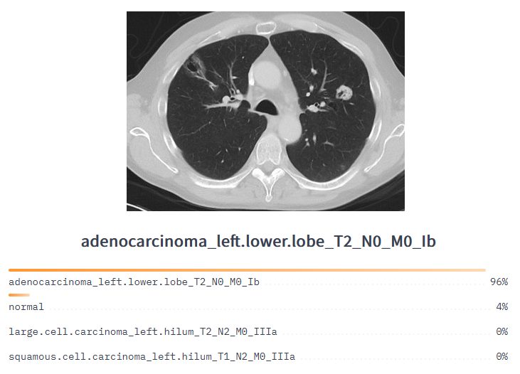
Medical Diagnosis: Since LNNs have a dynamic architecture, they can be used in medical diagnosis as they can adapt to new situations without expensive training. These healthcare use cases can include medical image analysis, health records analysis, and biomedical signal processing.
Self-Driving Cars: The dynamic architecture of LNNs has the potential to drastically improve the performance of self-driving cars. Sometimes AI models used in cars encounter data that is not part of their training data. The model doesn’t know what to do in this scenario and this can lead to accidents. LNNs can help avoid this as they learn on the job and adapt their behavior.

Natural language Processing (NLP): Training huge textual data using Conventional Neural Networks (CNNs) for sentiment analysis, entity recognition, etc., can be a time-consuming process requiring huge computational resources. LNNs solve this problem as they require fewer computational resources and can adapt to the incoming data without repeated training of the model.
What’s Next?
Liquid Neural Networks represent a new area of research that is still unexplored and has a lot of potential in various sectors. They offer a lot of benefits over traditional neural networks. However, they also have some drawbacks. Research is going on in this direction, and hopefully, one day, they may change the landscape of Artificial Intelligence.
If you want to learn more about the different types of networks and understand them, read the below blogs for further information.
- Introduction to Spatial Transformer Networks
- Capsule Networks: A New Approach to Deep Learning
- Graph Neural Networks (GNNs): A Comprehensive Guide
- Deep Belief Networks (DBNs) Explained
- Guide to Generative Adversarial Networks (GANs)