EfficientNet is a Convolutional Neural Network (CNN) architecture that utilizes a compound scaling method to uniformly scale depth, width, and resolution, providing high accuracy with computational efficiency.
CNNs (Convolutional Neural Networks) power computer vision tasks like object detection and image classification. Their ability to learn from raw images has led to breakthroughs in autonomous vehicles, medical diagnosis, and facial recognition. However, as the size and complexity of datasets grow, CNNs need to become deeper and more complex to maintain high accuracy.
Increasing the complexity of CNNs leads to better accuracy, which demands more computational resources.
This increased computational demand makes CNN impractical for real-time applications, and use on devices with limited processing capabilities (smartphones and IoT devices). This is the problem EfficientNet tries to solve. It provides a solution for sustainable and efficient scaling of CNNs.
The Path to EfficientNet
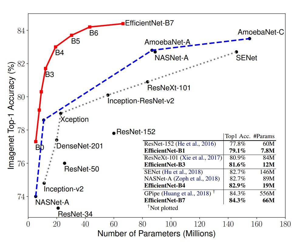
The popular strategy of increasing accuracy through growing model size yielded impressive results in the past, with models like GPipe achieving state-of-the-art accuracy on the ImageNet dataset.
From GoogleNet to GPipe (2018), ImageNet top-1 accuracy jumped from 74.8% to 84.3%, along with parameter counts (going from 6.8M to 557M), leading to excessive computational demands.
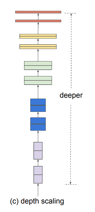
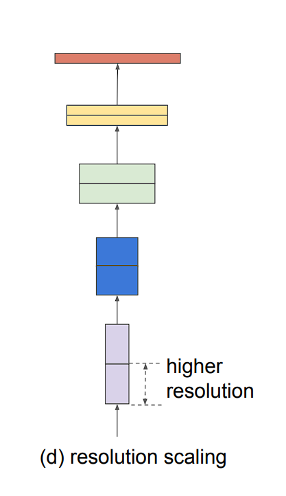
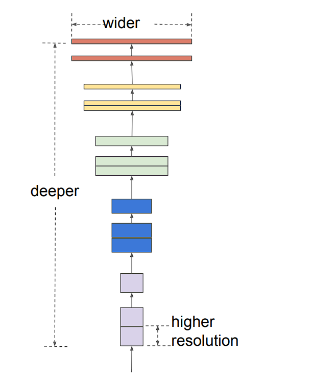
Model scaling can be achieved in three ways: by increasing model depth, width, or image resolution.
- Depth (d): Scaling network depth is the most commonly used method. The idea is simple, deeper ConvNet captures richer and more complex features and also generalizes better. However, this solution comes with a problem, the vanishing gradient problem.
- Width (w): This is used in smaller models. Widening a model allows it to capture more fine-grained features. However, extra-wide models are unable to capture higher-level features.
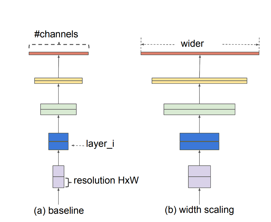
- Image resolution (r): Higher resolution images enable the model to capture more fine-grained patterns. Previous models used 224 x 224 size images, and newer models tend to use a higher resolution. However, higher resolution also leads to increased computation requirements.
Problem with Scaling
As we have seen, scaling a model has been a go-to method, but it comes with overhead computation costs. Here is why:
More Parameters: Increasing depth (adding layers) or width (adding channels within convolutional layers) leads to a significant increase in the number of parameters in the network. Each parameter requires computation during training and prediction. More parameters translate to more calculations, increasing the overall computational burden.
Moreover, scaling also leads to Memory Bottleneck as larger models with more parameters require more memory to store the model weights and activations during processing.
What is EfficientNet?
EfficientNet proposes a simple and highly effective compound scaling method, which enables it to easily scale up a baseline ConvNet to any target resource constraints, in a more principled and efficient way.
What is Compound Scaling?
The creator of EfficientNet observed that different scaling dimensions (depth, width, image size) are not independent.
High-resolution images require deeper networks to capture large-scale features with more pixels. Additionally, wider networks are needed to capture the finer details present in these high-resolution images. To pursue better accuracy and efficiency, it is critical to balance all dimensions of network width, depth, and resolution during ConvNet scaling.
However, scaling CNNs using particular ratios yields a better result. This is what compound scaling does.
The compound scaling coefficient method uniformly scales all three dimensions (depth, width, and resolution) in a proportional manner using a predefined compound coefficient ɸ.
Here is the mathematical expression for the compound scaling method:
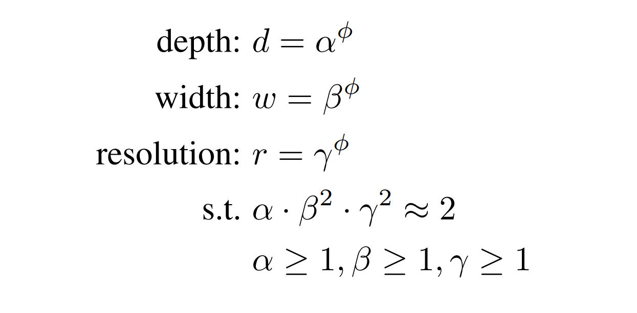
α: Scaling factor for network depth (typically between 1 and 2)
β: Scaling factor for network width (typically between 1 and 2)
γ: Scaling factor for image resolution (typically between 1 and 1.5)
ɸ (phi): Compound coefficient (positive integer) that controls the overall scaling factor.
This equation tells us how much to scale the model (depth, width, resolution) which yields maximum performance.
Benefits of Compound Scaling
- Optimal Resource Utilization: By scaling all three dimensions proportionally, EfficientNet avoids the limitations of single-axis scaling (vanishing gradients or saturation).
- Flexibility: The predefined coefficients allow for creating a family of EfficientNet models (B0, B1, B2, etc.) with varying capacities. Each model offers a different accuracy-efficiency trade-off, making them suitable for diverse applications.
- Efficiency Gains: Compared to traditional scaling, compound scaling achieves similar or better accuracy with significantly fewer parameters and FLOPs (FLoating-point Operations Per Second), making them ideal for resource-constrained devices.
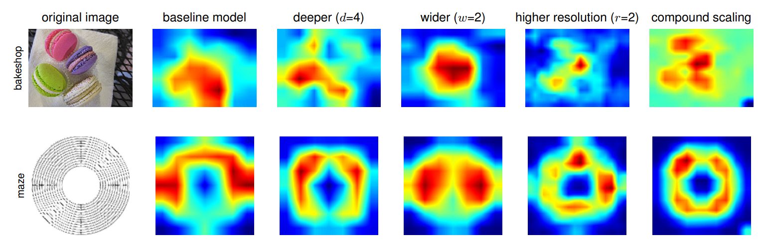
Moreover, we visualize the advantage of compound scaling using an activation map.
However, to develop an efficient CNN model that can be scaled, the creator of EfficientNet created a unique baseline network, called the EfficientNets. This baseline network is then further scaled in steps to obtain a family of larger networks (EfficientNet-B0 to EfficientNet-B7).
The EfficientNet Family
EfficientNet consists of 8 models, going from EfficientNet-B0 to EfficientNet-B7.
| Features | Top-1 Acc | Top-5 Acc | Params | FLOPs |
|---|---|---|---|---|
| EfficientNet-B0 | 77.1% | 93.3% | 5.3M | 0.39B |
| EfficientNet-B1 | 79.1% | 94.4% | 7.8M | 0.70B |
| EfficientNet-B2 | 80.1% | 94.9% | 9.2M | 1.0B |
| EfficientNet-B3 | 81.6% | 95.7% | 12M | 1.8B |
| EfficientNet-B4 | 82.9% | 96.4% | 19M | 4.2B |
| EfficientNet-B5 | 83.6% | 96.7% | 30M | 9.9B |
| EfficientNet-B6 | 84.0% | 96.8% | 43M | 19B |
| EfficientNet-B7 | 84.3% | 97.0% | 66M | 37B |
EfficientNet-B0 is the foundation upon which the entire EfficientNet family is built. It’s the smallest and most efficient model within the EfficientNet variants.
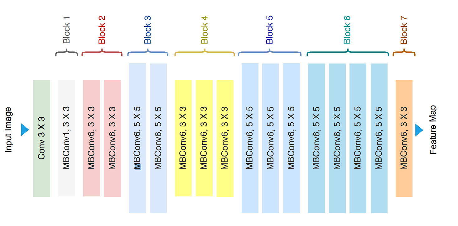
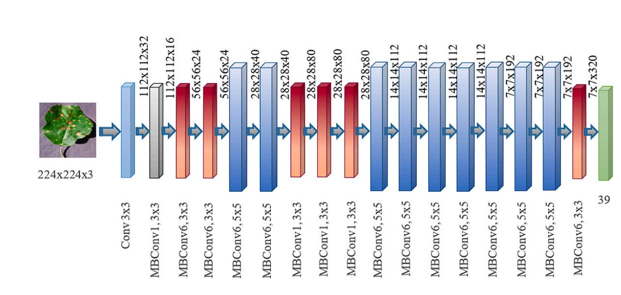
EfficientNet Architecture
EfficientNet-B0, discovered through Neural Architectural Search (NAS) is the baseline model. The main components of the architecture are:
- MBConv block (Mobile Inverted Bottleneck Convolution)
- Squeeze-and-excitation optimization
The MBConv Block
The MBConv block is an evolved inverted residual block inspired by MobileNetv2.
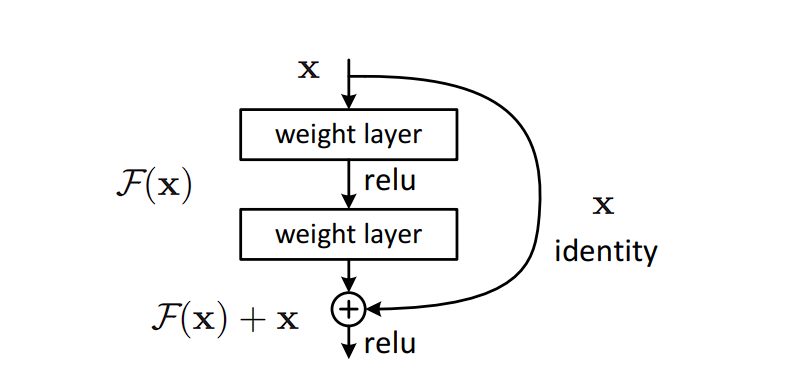
What is a Residual Network?
Residual networks (ResNets) are a type of CNN architecture that addresses the vanishing gradient problem, as the network gets deeper, the gradient diminishes. ResNets solves this problem and allows for training very deep networks. This is achieved by adding the original input to the output of the transformation applied by the layer, improving gradient flow through the network.
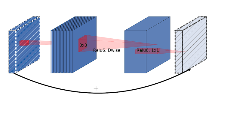
What is an inverted residual block?
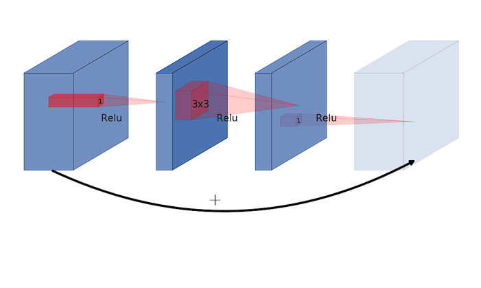
In residual blocks used in ResNets, the main pathway involves convolutions that reduce the dimensionality of the input feature map. A shortcut or residual connection then adds the original input to the output of this convolutional pathway. This process allows the gradients to flow through the network more freely.
However, an inverted residual block starts by expanding the input feature map into a higher-dimensional space using a 1×1 convolution then applies a depthwise convolution in this expanded space and finally uses another 1×1 convolution that projects the feature map back to a lower-dimensional space, the same as the input dimension. The “inverted” aspect comes from this expansion of dimensionality at the beginning of the block and reduction at the end, which is opposite to the traditional approach where expansion happens towards the end of the residual block.
What is Squeeze-and-Excitation?
Squeeze-and-Excitation (SE) simply allows the model to emphasize useful features, and suppress the less useful ones. We perform this in two steps:
- Squeeze: This phase aggregates the spatial dimensions (width and height) of the feature maps across each channel into a single value, using global average pooling. This results in a compact feature descriptor that summarizes the global distribution for each channel, reducing each channel to a single scalar value.
- Excitation: In this step, the model using a full-connected layer applied after the squeezing step, produces a collection of per channel weight (activations or scores). The final step is to apply these learned importance scores to the original input feature map, channel-wise, effectively scaling each channel by its corresponding score.
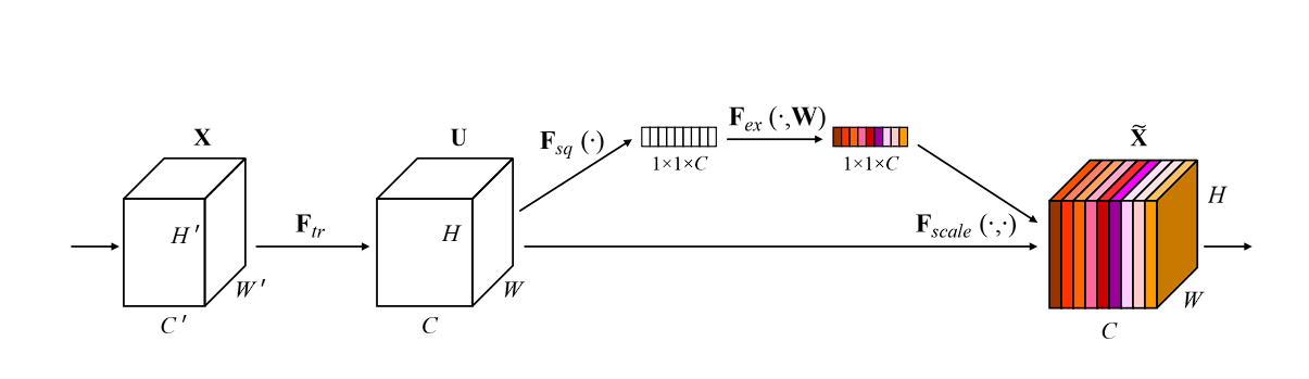
This process allows the network to emphasize more relevant features and diminish less important ones, dynamically adjusting the feature maps based on the learned content of the input images.
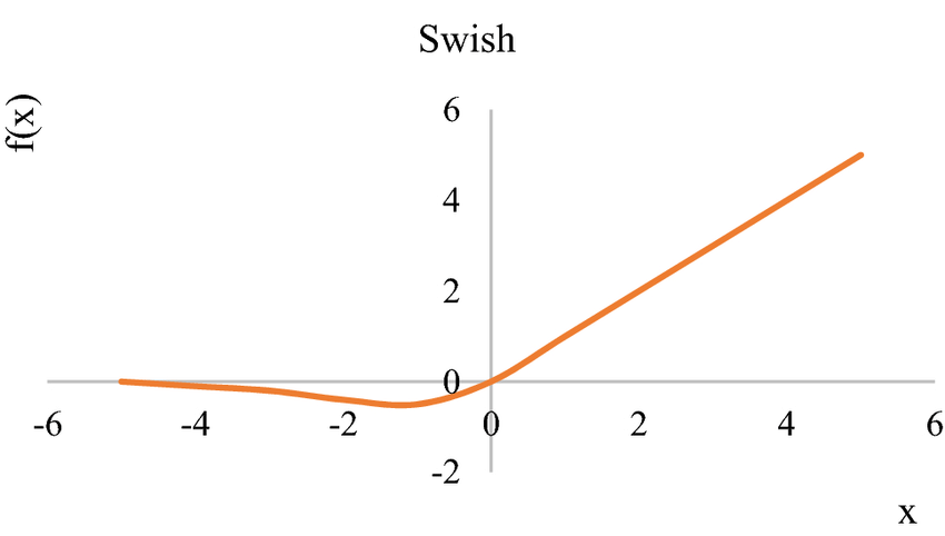
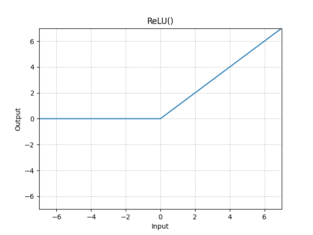
Moreover, EfficientNet also incorporates the Swish activation function as part of its design to improve accuracy and efficiency.
What is the Swish Activation Function?
Swish is a smooth continuous function, unlike Rectified Linear Unit (ReLU) which is a piecewise linear function. Swish allows a small number of negative weights to be propagated through, while ReLU thresholds all negative weights to zero.
EfficientNet incorporates all the above elements into its architecture. Finally, the architecture looks like this:
| Stage
i |
Operator
^Fi |
Resolution
^Hi x ^Wi |
#Channels
^Ci |
#Layers
^Li |
|---|---|---|---|---|
| 1 | Conv3x3 | 224 x 224 | 32 | 1 |
| 2 | MBConv1, k3x3 | 112 x 112 | 16 | 1 |
| 3 | MBConv6, k3x3 | 112 x 112 | 24 | 2 |
| 4 | MBConv6, k5x5 | 56 x 56 | 40 | 2 |
| 5 | MBConv6, k3x3 | 28 x 28 | 80 | 3 |
| 6 | MBConv6, k5x5 | 14 x 14 | 112 | 3 |
| 7 | MBConv6, k5x5 | 14 x 14 | 192 | 4 |
| 8 | MBConv6, k3x3 | 7 x 7 | 320 | 1 |
| 9 | Conv1x1 & Pooling & FC | 7 x 7 | 1280 | 1 |
EfficientNet Architecture.
Performance and Benchmarks of EfficientNet
The EfficientNet family, from EfficientNet-B0 to EfficientNet-B7 and beyond, offers a range of complex and accurate models. Here are some key performance benchmarks for EfficientNet on the ImageNet dataset, reflecting the balance between efficiency and accuracy.
The benchmarks obtained are performed on the ImageNet dataset. Here are a few key insights from the benchmark:
- Higher accuracy with fewer parameters: EfficientNet models achieve high accuracy with fewer parameters and lower FLOPs than other convolutional neural networks (CNNs). For example, EfficientNet-B0 achieves 77.1% top-1 accuracy on ImageNet with only 5.3M parameters, while ResNet-50 achieves 76.0% top-1 accuracy with 26M parameters. Additionally, the B-7 model performs at par with Gpipe, but with way fewer parameters ( 66M vs 557M).
- Fewer Computations: EfficientNet models can achieve similar accuracy to other CNNs with significantly fewer FLOPs. For example, EfficientNet-B1 achieves 79.1% top-1 accuracy on ImageNet with 0.70 billion FLOPs, while Inception-v3 achieves 78.8% top-1 accuracy with 5.7 billion FLOPs.
As the EfficientNet model size increases (B0 to B7), the accuracy and FLOPs also increase. However, the increase in accuracy is smaller for the larger models. For example, EfficientNet-B0 achieves 77.1% top-1 accuracy, while EfficientNet-B7 achieves 84.3% top-1 accuracy.
| Model | Top-1 Acc. | Top-5 Acc. | #Params | Ratio-to-EfficientNet | #FLOPs | Ratio-to-EfficientNet |
|---|---|---|---|---|---|---|
| EfficientNet-B0 | 77.1% | 93.3% | 5.3M | 1x | 0.39B | 1x |
| ResNet-50 (He et al., 2016) | 76.0% | 93.0% | 26M | 4.9x | 4.1B | 11x |
| DenseNet-169 (Huang et al., 2017) | 76.2% | 92.3% | 14M | 2.6x | 3.5B | 8.9x |
| EfficientNet-B1 | 79.1% | 94.4% | 7.8M | 1x | 0.70B | 1x |
| ResNet-152 (He et al., 2016) | 77.8% | 93.8% | 60M | 76.x | 11B | 16x |
| DenseNet-264 (Huang et al., 2017) | 77.9% | 93.9% | 34M | 4.3x | 6.0B | 8.6x |
| Inception-v3 (Szegedy et al., 2016) | 78.8% | 94.4% | 24M | 3.0x | 5.7B | 8.1x |
| Xception (Chollet, 2017) | 79.0% | 94.5% | 23M | 3.0x | 8.4B | 12x |
| EfficientNet-B2 | 80.1% | 94.9% | 9.2M | 1x | 1.0B | 1x |
| Inception-v4 (Szegedy et al., 2017) | 80.0% | 95.0% | 48M | 5.2x | 13B | 13x |
| Inception-resnet-v2 (Szegdy et al., 2017) | 80.1% | 95.1% | 56M | 6.1x | 13B | 13x |
| EfficientNet-B3 | 81.6% | 95.7% | 12M | 1x | 1.8B | 1x |
| ResNeXt-101 (Xie et al., 2017) | 80.9% | 95.6% | 84M | 7.0x | 32B | 18x |
| PolyNet (Zhang et al., 2017) | 81.3% | 95.8% | 92M | 7.7x | 35B | 19x |
| EfficientNet-B4 | 82.9% | 96.4% | 19M | 1x | 4.2B | 1x |
| SENet (Hu et al., 2018) | 82.7% | 96.2% | 146M | 7.7x | 42B | 10x |
| NASNet-A (Zoph et al., 2018) | 82.7% | 96.2% | 89M | 4.7x | 24B | 5.7x |
| AmoebaNet-A (Real et al., 2019) | 82.8% | 96.2% | 87M | 4.6x | 23B | 5.5x |
| PNASNet (Liu et al., 2018) | 82.9% | 96.2% | 86M | 4.5x | 23B | 6.0x |
| EfficientNet-B5 | 83.6% | 96.7% | 30M | 1x | 9.9B | 1x |
| AmoebaNet-C (Cubuk et al., 2019) | 83.5% | 96.5% | 155M | 5.2x | 41B | 4.1x |
| EfficientNet-B6 | 84.0% | 96.8% | 43M | 1x | 19B | 1x |
| EfficientNet-B7 | 84.3% | 97.0% | 66M | 1x | 37B | 1x |
| GPipe (Huang et al., 2018) | 84.3% | 97.0% | 557M | 8.4x | – | – |
EfficientNet Benchmark.
Applications Of EfficientNet
EfficientNet’s strength lies in its ability to achieve high accuracy while maintaining efficiency. This makes it an important tool in scenarios where computational resources are limited. Here are some of the use cases for EfficientNet models:
- Human Emotion Analysis on Mobile Devices: Video-based facial analysis of the affective behavior of humans done using the EfficientNet model on Mobile Devices, which achieved an F1-score of 0.38. Read here.

- Health and Medicine: Use of B0 model for cancer diagnosis which obtained an accuracy of 91.18%.
- Plant Leaf disease: Plant leaf disease classification done using a deep learning model showed that the B5 and B4 models of EfficientNet architecture achieved the highest values compared to other deep learning models in original and augmented datasets with 99.91% for accuracy and 99.39% for precision respectively.
- Mobile and Edge Computing: EfficientNet’s lightweight architecture, especially the B0 and B1 variants, makes it perfect for deployment on mobile devices and edge computing platforms with limited computational resources. This allows EfficientNet to be used in real-time applications like augmented reality, enhancing mobile photography, and performing real-time video analysis.
- Embedded Systems: EfficientNet models can be used in resource-constrained embedded systems for tasks like image recognition in drones or robots. Their efficiency allows for on-board processing without requiring powerful hardware.
- Faster Experience: EfficientNet’s efficiency allows for faster processing on mobile devices, leading to a smoother user experience in applications like image recognition or augmented reality, moreover with reduced battery consumption.
Further Reads for EfficientNet
To learn more about the world of machine learning and computer vision, we encourage you to check out our other viso.ai blogs:
- Real-time Computer Vision: AI at the Edge
- Deep Neural Networks: 3 Popular Types (CNNs, ANNs, MLPs)
- Hardware at the Edge: Google Coral TPU
- An Exhaustive Guide to OpenVINO
- Introducing Mask R CNN for Engineers, Practitioners, Data Scientists, and Researchers