Representation Learning is a process that simplifies raw data into understandable patterns for machine learning. It enhances interpretability, uncovers hidden features, and aids in transfer learning.
Data in its raw form (words and letters in text, pixels in images) is too complex for machines to process directly. Representation learning transforms the data into a representation that machines can use for classification or predictions.
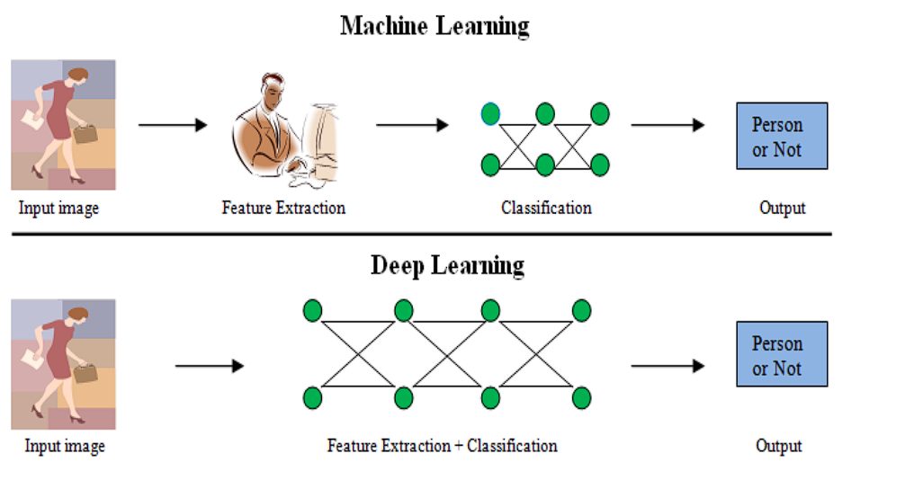
Deep Learning, a subset of Machine Learning tasks has been revolutionary in the past two decades. This success of Deep Learning heavily relies on the advancements made in representation learning.
Previously, manual feature engineering constrained model capabilities, as it required extensive expertise and effort to identify relevant features. Whereas Deep learning automated this feature extraction.
History of Representation Learning
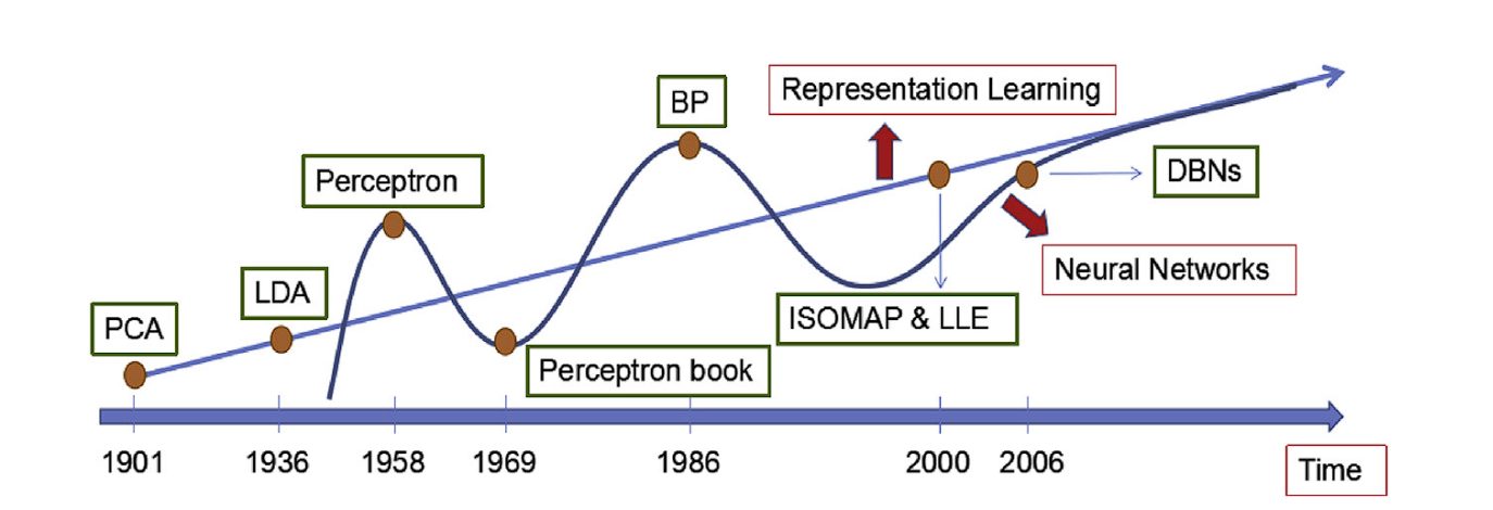
Representation Learning has advanced significantly. Hinton and co-authors’ breakthrough discovery in 2006 marks a pivotal point, shifting the focus of representation learning towards Deep Learning Architectures. The researchers’ concept of employing greedy layer-wise pre-training followed by fine-tuning deep neural networks led to further developments.
Here is a quick overview of the timeline.
- Traditional Techniques (Pre-2000):
- Linear Methods:
- Principal Component Analysis (PCA): Focuses on capturing overall data variance for dimensionality reduction.
- Linear Discriminant Analysis (LDA): Emphasizes maximizing separation between classes in the low-dimensional space.
- Kernel: Researchers created techniques like Kernel PCA to manage non-linear data by projecting it into a higher-dimensional space before applying linear methods.
- Manifold Learning (2000’s): This approach emerged to discover the intrinsic low-dimensional structure (manifold) hidden within high-dimensional data.

Dimensionality Reduction – Source
- Linear Methods:
- Deep Learning Era (2006 onwards):
- Neural Networks: The introduction of deep neural networks by Hinton et al. in 2006 marked a turning point. Deep Neural Network models could learn complex, hierarchical representations of data through multiple layers. Eg, CNN, RNN, Autoencoder, and Transformers.

What is a Good Representation?
A good representation has three characteristics: Information, compactness, and generalization.
- Information: The representation encodes important features of the data into a compressed form.
- Compactness:
- Low Dimensionality: Learned embedding representations from raw data should be much smaller than the original input. This allows for efficient storage and retrieval, and also discards noise from the data, allowing the model to focus on relevant features and converge faster.
- Preserves Essential Information: Despite being lower-dimensional, the representation retains important features. This balance between dimensionality reduction and information preservation is essential.
- Generalization (Transfer Learning): The aim is to learn versatile representations for transfer learning, starting with a pre-trained model (computer vision models are often trained on ImageNet first) and then fine-tuning it for specific tasks requiring less data.
Deep Learning for Representation Learning
Deep Neural Networks are representation learning models. They encode the input information into hierarchical representations and project it into various subspaces. These subspaces then go through a linear classifier that performs classification operations.
Deep Learning tasks can be divided into two categories: Supervised and Unsupervised Learning. The deciding factor is the use of labeled data.
- Supervised Representation Learning:
- Leverages Labeled Data: Uses labeled data. The labels guide the learning algorithm about the desired outcome.
- Focuses on Specific Tasks: The learning process is tailored towards a specific task, such as image classification or sentiment analysis. The learned representations are optimized to perform well on that particular task.
- Examples:
- Training a Convolutional Neural Network (CNN) to classify objects in images (e.g., dog, cat) using labeled image datasets, or a Recurrent Neural Network (RNN) for sentiment analysis of text data (positive, negative, neutral) with labeled reviews or sentences.
- Unsupervised Representation Learning:
- Without Labels: Works with unlabeled data. The algorithm identifies patterns and relationships within the data itself.
- Focuses on Feature Extraction: The goal is to learn informative representations that capture the underlying structure and essential features of the data. These representations can then be used for various downstream tasks (transfer learning).
- Examples:
- Training an autoencoder to compress and reconstruct images, learning a compressed representation that captures the key features of the image.
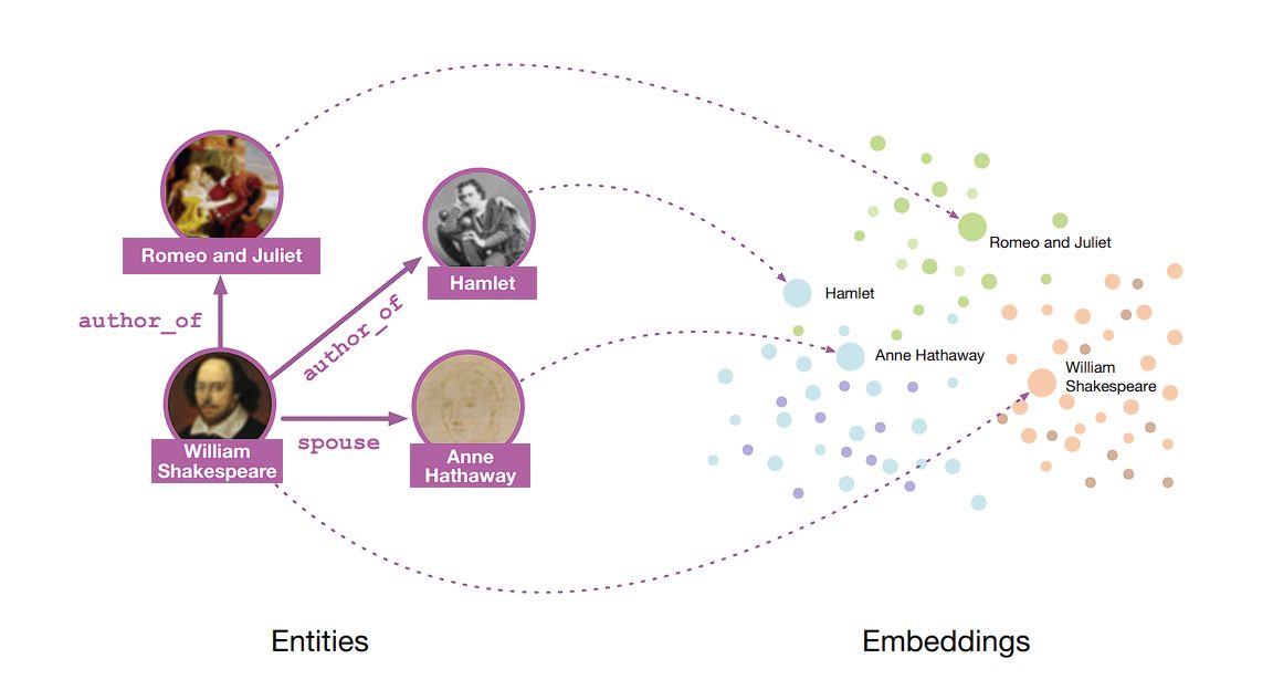
- Using Word2Vec or GloVe on a massive text corpus to learn word embeddings, where words with similar meanings have similar representations in a high-dimensional space.
- BERT to learn contextual representation of words.
Supervised Deep Learning
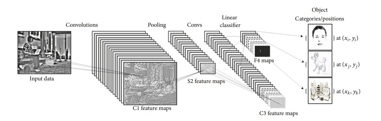
Convolutional Neural Networks (CNNs)
CNNs are a class of supervised learning models that are highly effective in processing grid-like structured data (images).
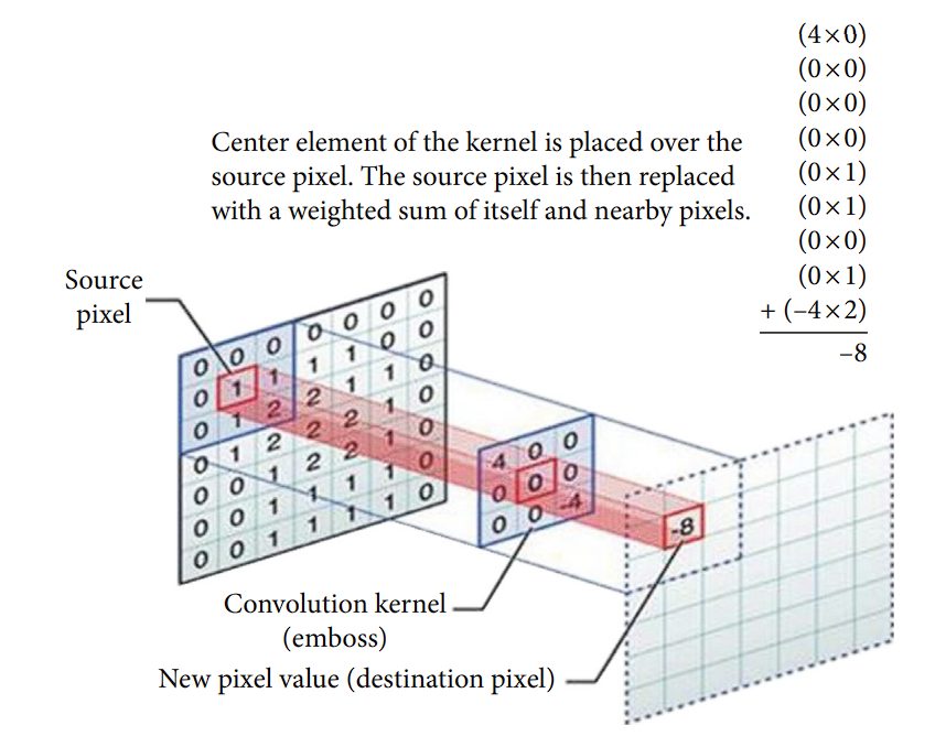
A CNN captures the spatial and temporal dependencies in an image through the application of learnable filters or kernels. The key components of CNNs include:
- Convolutional Layers: These layers apply filters to the input to create feature maps, highlighting important features like edges and shapes.
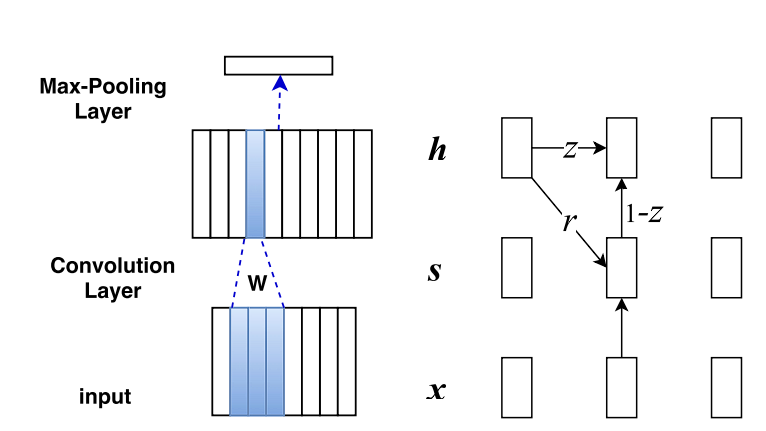
- Pooling Layers: Follow convolutional layers to reduce the dimensionality of the feature maps, making the model more efficient by retaining only the most essential information.
- Fully Connected Layers: At the end of the network, these layers classify the image based on the features extracted by the convolutional and pooling layers.
CNNs are good at learning hierarchical feature representations in images. Lower layers learn to detect edges, colors, and textures, while deeper layers identify more complex structures like parts of objects or entire objects themselves. This hierarchical learning approach is highly effective for tasks requiring the recognition of complex patterns and objects within images.
CNNs provide translation invariance. This means, that even if an object moves around in an image, or the image is rotated, or skewed, it can still recognize the image. Moreover, the learned filters incorporate large number parameter sharing, allowing for dense and reduced size representation.
Recurrent Neural Networks (RNNs)
Recurrent Neural Networks (RNNs) and their variants, including Long Short-Term Memory (LSTM) networks and Gated Recurrent Units (GRUs), specialize in processing sequential data, making them highly suitable for tasks in natural language processing and time series analysis.
The core idea behind RNNs is their ability to maintain a memory of previous inputs in their internal state, which influences the processing of current and future inputs, allowing them to capture temporal dependencies.
- RNNs possess a simple structure where the output from the previous step is fed back into the network as input for the current step, creating a loop that allows information to persist. However, they suffer from exploding and vanishing gradients.
- LSTMs are an advanced variant of RNN. They introduce a complex architecture with a memory cell and three gates (input, forget, and output gates). These components work together to regulate the flow of information, deciding what to retain in memory, what to discard, and what to output. Which solves the exploding and vanishing gradients problem.
- GRUs simplify the LSTM design by combining the input and forget gates into a single “update gate” and merging the cell state and hidden state.
However, RNNs, LSTMs, and GRUs learn to capture temporal dependencies by adjusting their weights by backpropagation through time (BPTT), a variant of the standard backpropagation algorithm adapted for sequential data.
By doing so, these networks learn complex patterns in the data, such as the grammatical structure in a sentence or trends in a time series, effectively capturing both short-term and long-term dependencies.
Unsupervised Deep Learning
Autoencoders
Autoencoders, as unsupervised feature learning models, learn encodings of unlabeled data, usually for dimensionality reduction or feature learning. Essentially, they aim to reconstruct input data from the constructed representation.
Autoencoders have two parts, encoder and decoder.
- Encoder: The encoder compresses the input into a latent-space representation. It learns to reduce the dimensionality of the input data, capturing its most important features in a compressed form.
- Decoder: The decoder takes the encoded data and tries to recreate the original input. The reconstruction might not be perfect but with training, the decoder learns to produce output significantly similar to the input.
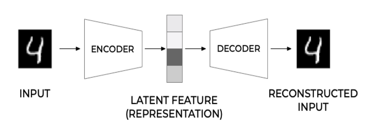
Auto-encoders learn to create dense and useful representations of data by forcing the network to prioritize important aspects of the input data. These learned representations can be later used for various other tasks.
Variational Autoencoders (VAEs)
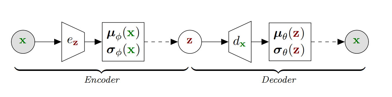
Variational Autoencoders (VAEs) are a unique kind of autoencoder that compresses data probabilistically, unlike regular autoencoders. Instead of converting an input (e.g. an image) into a single compressed form, VAEs transform it into a spectrum of possibilities within the latent space, often represented by a multivariate Gaussian distribution.
Thus, when compressing an image, VAEs don’t select a specific point in the latent space but rather a region that encapsulates the various interpretations of that image. Upon decompression, VAEs reconvert these probabilistic mappings into images, enabling them to generate new images based on learned representations.
Here are the steps involved:
- Encoder: The encoder in a VAE maps the input data to a probability distribution in the latent space. It produces two things for each input: a mean (μ) and a variance (σ²), which together define a Gaussian distribution in the latent space.
- Sampling: Instead of directly passing the encoded representation to the decoder, VAEs sample a point from the Gaussian distribution defined by the parameters produced by the encoder. This sampling step introduces randomness into the process, which is crucial for the generative aspect of VAEs.
- Decoder: The sampled point is then passed to the decoder, which attempts to reconstruct the original input from this sampled latent representation. The reconstruction will not be perfect, partly because of the randomness introduced during sampling, but it will be similar to the original input.
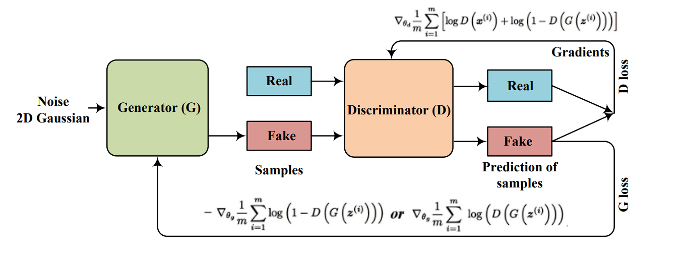
Generative Adversarial Networks (GANs)
Generative Adversarial Networks (GANs), introduced by Ian Goodfellow and colleagues in 2014, are a type of artificial intelligence algorithm used in unsupervised machine learning.
They involve two neural networks: the generator, which aims to create data resembling real data, and the discriminator, which tries to differentiate between real and generated data. These networks are trained together in a competitive game-like process.
- Generator: The generator network takes random noise as input and generates samples that resemble the distribution of the real data. Its goal is to produce data so convincing that the discriminator cannot tell it apart from actual data.
- Discriminator: The discriminator network is a classifier that tries to distinguish between real data and fake data produced by the generator. It is trained on a mixture of real data and the fake data generated by the generator, learning to make this distinction.
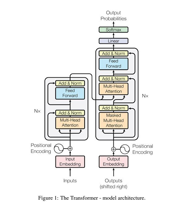
Transformers
Transformers have revolutionized natural language processing (NLP), offering significant improvements over previous models like RNNs and LSTMs for tasks like text translation, sentiment analysis, and question-answering.
The core innovation of the Transformer is the self-attention mechanism, which allows the model to weigh the importance of different parts of the input data differently, enabling it to learn complex representations of sequential data.
A Transformer model is composed of an encoder and a decoder, each consisting of a stack of identical layers.
- Encoder: Processes the input data (e.g., a sentence) and transforms it into a continuous representation that holds the learned information of that input.
- Decoder: Takes the encoder’s output and generates the final output sequence, step by step, using the encoder’s representation and what it has produced so far.
Both the encoder and decoder are made up of multiple layers that include self-attention mechanisms.
Self-Attention is the ability of the model to associate each word in the input sequence with every other word to better understand the context and relationships within the data. It calculates the attention scores, indicating how much focus to put on other parts of the input sequence when processing a specific part.
Unlike sequential models like RNNs, the Transformer treats input data as a whole, allowing it to capture context from both directions (left and right of each word in NLP tasks) simultaneously. This leads to more nuanced and contextually rich representations.
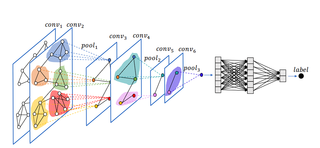
Graph Neural Networks
Graph Neural Networks (GNNs) are designed to perform representation learning on graph-structured data.
The main idea behind GNNs is to learn a representation (embedding) for each node and edge, which captures the node’s attributes and the structural information of its neighborhood. The core component of GNNs is message passing. By stacking multiple message-passing layers, GNNs capture immediate neighbor information and features from the neighborhood.
This results in node embeddings or representations that reflect both local graph topology and global structure. The final node embeddings can then be used for various tasks such as node classification, link prediction, and graph classification.
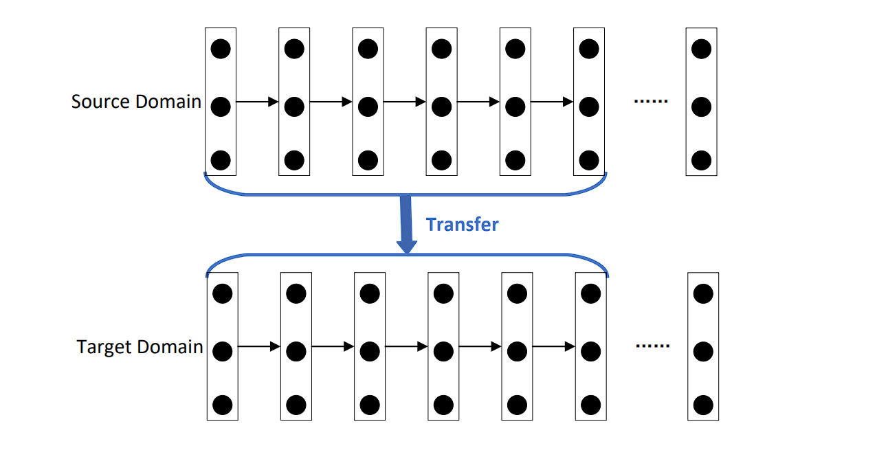
Transfer Learning
In transfer learning, you first train a model on a very large and comprehensive dataset. This initial training allows the model to learn a rich representation of features, weights, and biases. Then, you use this learned representation as a starting point for a second model, which may not have as much training data available.
For instance, in the field of computer vision, models often undergo pre-training on the ImageNet dataset, which includes over a million annotated images. This process helps the model to learn rich features.
Furthermore, after this pre-training phase, you can fine-tune the model on a smaller, task-specific dataset. During this fine-tuning phase, the model adapts the general features it learned during pre-training to the specifics of the new task.
Applications of Representation Learning
Computer Vision
- Feature Extraction: In traditional computer vision techniques, feature extraction was a manual process, however DL-based models like CNNs streamlined feature extraction. CNNs and Autoencoders perform edge detection, texture analysis, or color histograms by themselves.
- Generalization and Transfer Learning: Representation Learning has facilitated the creation of robust models like YOLO and EfficientNet for object detection, and semantic segmentation.
Natural Language Processing (NLP)
- Language Models: NLP models like BERT and GPT use representation learning to understand the context and semantics of words in sentences, significantly improving performance on tasks like text classification, sentiment analysis, machine translation, and question answering.
- Word Embeddings: Techniques like Word2Vec and GloVe learn dense vector representations of words based on their co-occurrence information, capturing semantic similarity and enabling improved performance in almost all NLP tasks.
Audio and Speech Processing
- Speech Recognition: Speech Recognition utilizes representation learning to transform raw audio waveforms into informative features. These features capture the essence of phonetics and language, ultimately enabling accurate speech-to-text conversion.
- Music Generation: Models learn representations of musical patterns, and then generate new pieces of music that are stylistically consistent with the training data.
Healthcare
- Disease Diagnosis: Representation learning extracts meaningful features from medical images (like X-rays, and MRIs) or electronic health records, assisting in the diagnosis of diseases such as cancer.
- Genomics: Learning representations of genetic sequences aids in understanding gene function, predicting gene expression levels, and identifying genetic markers associated with diseases.
What’s Next?
Get started with enterprise-grade computer vision. Viso Suite allows ML teams to seamlessly integrate computer vision into their workflows in a matter of days – drastically shortening the time-to-value of the application. Learn more by booking a demo with us.
