
In today’s digital world, Artificial Intelligence (AI) and Machine learning (ML) models are used everywhere, from face detection in electronic devices to real-time language translation. Efficient, quick, and cost-effective learning processes are crucial for scaling these models.
Transfer Learning is a key technique implemented by researchers and ML scientists to enhance efficiency and reduce costs in Deep learning and Natural Language Processing.
What is Transfer Learning?
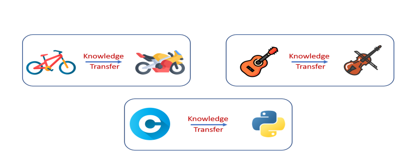
As the name suggests, this technique involves transferring the learnings of one trained machine learning model to another, in the form of neural network weights. This provides a significant edge to businesses as they don’t need to train a model from scratch. For example, to train a model to translate German movie subtitles to English, we usually have to train it with thousands of German and English text corpora, so that it can understand and translate.
But, there are open source models like German-BERT that are already trained on huge data corpora, with many parameters. Through transfer learning, the representation learning of German-BERT is utilized, and additional subtitle data is provided. Let us understand how this works.
To understand how transfer learning works, it is essential to understand the architecture of Deep Neural Networks. Neural Networks are the most widely used algorithm to build ML models for many advanced tasks, as they have shown higher performance accuracy than traditional algorithms.
Understanding Neural Networks
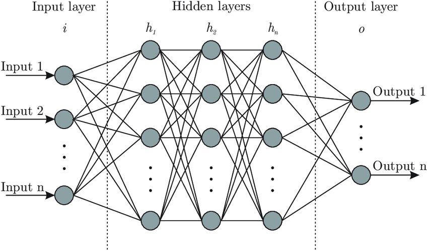
Any neural network architecture consists of 3 main parts: the input layer, multiple hidden layers, and the output.
The hidden layers have neurons, which are initialized with random weights at the beginning. During training, we supply the input variables to the input layer. Then the layers of the neural network extract features, learn data patterns, and update their weights. At the end of training, all units would have learned the weights and can make predictions.
Transfer Learning in Neural Networks
The main hurdle in implementing neural networks is the long training time and computational costs incurred. The process would be much quicker if we could retain the learned weights of a model (also referred to as ‘pre-trained weights’), and re-use them for a similar use case. This is where transfer learning comes into play.
In transfer learning, we initialize the neurons with pre-trained weights, rather than random ones. The base model leveraged for the learned weights is called the ‘Pre-trained Model’, and is usually trained with heavy parameters.
There are many such pre-trained models available in open source, and also some that require paid subscriptions. Some common free-to-use pre-trained models include BERT, ResNet, YOLO etc.
The Necessity of Transfer Learning
Transfer learning can help solve many challenges faced during real-time ML model building. Some of them include:
- Reduction in Data Reliance: Several man-hours needed to collect high-quality data can be saved through transfer learning. We can also avoid the efforts required in annotation to create labels manually. We can take a pre-trained model and fine-tune it on small datasets.
- Domain Adaptation: Consider a domain in a niche area, for example analyzing financial reports and summarizing the key points. If we train the model from scratch, it would take a lot of time for it to learn the basics. With a pre-trained model, this would already be taken care of. We can utilize this time to fine-tune it on domain-specific terms (KPIs etc.).
- Cost and Resource Reduction: Every ML team wants to build an affordable and reliable model. Teams can’t afford to burn cash on computational resources for all the tasks. With transfer learning, the memory and GPU clusters needed are reduced, decreasing storage and cloud computation costs.
- Avoiding Overfitting: In many domains, like credit risk and healthcare, data is often limited for small-scale companies or startups. In such cases, the model often overfits the training data sample. This leads to poor generalization towards unseen data. This problem can be mitigated by leveraging transfer learning.
- Incremental Learning Support: The model’s performance can be iteratively improved by fine-tuning it to cover the gaps. This can be very helpful when the model is running in real time. Because, the data distributions may change over periods, or due to seasonality spikes, etc.
- Promotion of R&D: Transfer learning accelerates R&D in ML as it provides a base to start. Researchers can focus on specific aspects of a problem without restarting from scratch. Examples include LLMs to provide news summaries with diverse perspectives, etc.
How Transfer Learning Works
Let us understand how transfer learning works with a practical example. Consider a scenario in which we are analyzing traffic surveillance, and want to find out which vehicles are the most common. For this, we would need a deep learning model that can classify a given input image into a category of vehicle.
The vehicle categories could be “Sedan”, “SUV”, “Truck”, “Two-wheeler”, “Commercial trucks”, etc. Now, let’s see how to build a model for this quickly using transfer learning.
Step 1: Choose a Pre-trained Model
First, we choose the base model, whose pre-trained weights will be leveraged. There are many open-source and paid options available for pre-trained models. Huggingface is a great platform to find open-source models, and OpenAI is one of the best paid options.
The base model should be trained on the same data type as the current dataset. If we are working with images, then we need to look for a model trained on many images, like ResNet or VGG.
We can choose a language model like BERT that can parse human text to build an NLP model, such as a text summary. Next, we need to look for models that are trained for similar objectives to the current task. For example, if you have a text-based sentiment classification task at hand, choosing a model trained for text classification can be helpful.
For our task, we will be using the VGG16 pre-trained model. VGG16 has a CNN (Convolutional Neural Network) based architecture that has 16 layers. It is trained on the “ImageNet” dataset, which has several images in all categories like birds, fruits, cars, animals, etc. Since it is trained on a vast dataset, it can quickly pick up the initial low-level feature representations of an input image like edges, shapes, and so on.
Step 2: Pre-process your fine-tuning data
The base model (pre-trained model) is coded to accept inputs in a specific format, depending on the architecture. The fine-tuning dataset needs to be converted into the same format so that it is compatible. For example, language models usually take input text in the form of tokens or vector embeddings. Whereas, image recognition models accept inputs in the format of pixels or Pytorch tensors.
For our task, VGG16 requires input images in the format of 224 x 224 pixels. So, we resize the images in our custom training data uniformly. Let’s also normalize the images, either to a standard 0–1 range or using mean and variance. This will help in providing better stability during model training.
Data augmentation techniques can be used to increase the fine-tuning data size or add more variation to the sample. A few common techniques for images include creating crop variations or performing flips and rotations. Note that pre-processing is the stage where we can ensure the model will be robust after training, by cleaning up noise and ensuring diversity in the sample.
Step 3: Adapting the model
Next, we need to train our custom dataset on top of the base model. There are two ways to approach this: Feature extraction and Fine-tuning.
Feature extraction: In this approach, we take the pre-trained model without any changes and use it as a feature extractor. The pre-trained model will extract the features from the input based on its learned weights. Then, we build a new classification model, where we provide these extracted features as input. It is a cost-effective method, as we are not making any changes in the layers of the pre-trained model.
Fine-tuning: In this method, along with the additional classifier layer on top, we also re-train a few upper layers of the base model. The weights are frozen on the deep layers so that learned features are not lost. Fine-tuning will provide better performance accuracy, as it gets trained on the custom data.
In cases where the domain data has its specific nuances, like medical images and financial risk assessment, fine-tuning is the better choice. The downside of fine-tuning is relatively higher costs than feature extraction from pre-trained models.
We can choose one among these approaches based on some critical factors: domain requirements and sensitivity level of tasks, affordability, and availability of sufficient data for fine-tuning.
For our task of vehicle image classification, we can go with the feature extraction method as VGG16 is already exposed to images of cars and other vehicles. Let us freeze the weights of all pre-trained layers in VGG16. These layers will extract features from the input images we provide.
Step 4: Train on custom data & evaluate
Based on the choice in the previous step, new data needs to be trained accordingly. We can fine-tune the parameters like the learning rate and batch size of the new classifier layer to get the best results. A high learning rate might often lead to overfitting, while a low learning rate will waste resources.
We also need to define the loss function that best represents the task at hand. During training, the objective of the model is to minimize the loss function. There are also different techniques to optimize the loss function, like Stochastic Gradient Descent, RMSProp (Root Mean Square Propagation), and Adam.
Once training is complete, the model can be evaluated on a set of unseen test images. If there is any repetition in the training and test samples, then the model will not generalize well.
As our task is an image classification task, we can go with cross-entropy as the loss function. It is a common choice in multi-class classification projects. We can choose the Adam optimizer (Adaptive Moment Estimation), as it offers better regularization. We can also create a confusion matrix of the test data results to see how well the model classifies different vehicle categories.
Implementing Transfer Learning using PyTorch
First, start by importing the necessary Python packages. PyTorch will be used for building and training the neural network, torch-vision will be used to load and preprocess the data, and numpy will be used for numerical operations.
# Import packages and modules
import torch
import torch.nn as nn
import torch.optim as optim
from torch.optim import lr_scheduler
import numpy as np
import torchvision
from torchvision import datasets, models, transforms
import matplotlib.pyplot as plt
import time
import os
Next, define data transformations and load the dataset. We use transformations such as resizing, cropping, and normalization. This section also involves splitting the dataset into training and validation sets.
# Define data transforms
data_transforms = {
    'train': transforms.Compose([
        transforms.RandomResizedCrop(224),
        transforms.RandomHorizontalFlip(),
        transforms.ToTensor(),
        transforms.Normalize([0.485, 0.456, 0.406], [0.229, 0.224, 0.225])
    ]),
    'val': transforms.Compose([
        transforms.Resize(256),
        transforms.CenterCrop(224),
        transforms.ToTensor(),
        transforms.Normalize([0.485, 0.456, 0.406], [0.229, 0.224, 0.225])
    ]),
}

# Set data directory
data_dir = 'path/to/your/dataset'

# Load dataset
image_datasets = {x: datasets.ImageFolder(os.path.join(data_dir, x), data_transforms[x])
                  for x in ['train', 'val']}

# Create dataloaders
dataloaders = {x: torch.utils.data.DataLoader(image_datasets[x], batch_size=4, shuffle=True, num_workers=4)
               for x in ['train', 'val']}

# Get dataset sizes
dataset_sizes = {x: len(image_datasets[x]) for x in ['train', 'val']}
class_names = image_datasets['train'].classes
Next, we need to load the pre-trained VGG16 model from the torch-vision models. We freeze the parameters of the pre-trained layers and modify the final fully connected layer to match the number of classes in our dataset.
# Loading the pre-trained base model
model_ft = models.vgg16(pretrained=True)

# Freeze parameters of pre-trained layers
for param in model_ft.parameters():
    param.requires_grad = False

# Modify the classifier
num_ftrs = model_ft.classifier[6].in_features
model_ft.classifier[6] = nn.Linear(num_ftrs, len(class_names))

# Define loss function and optimizer
criterion = nn.CrossEntropyLoss()
optimizer_ft = optim.SGD(model_ft.parameters(), lr=0.001, momentum=0.9)

# Decay LR by a factor of 0.1 every 7 epochs
exp_lr_scheduler = lr_scheduler.StepLR(optimizer_ft, step_size=7, gamma=0.1)
Here’s the basic framework to train the model using a loss function, optimizer, and scheduler. Changes can be made as per requirements.
def train_model(model, criterion, optimizer, scheduler, num_epochs=25):
    since = time.time()

    best_model_wts = model.state_dict()
    best_acc = 0.0

    for epoch in range(num_epochs):
        print('Epoch {}/{}'.format(epoch, num_epochs - 1))
        print('-' * 10)

        # Each epoch has a training and validation phase
        for phase in ['train', 'val']:
            if phase == 'train':
                model.train()  # Set model to training mode
            else:
                model.eval()   # Set model to evaluate mode

            running_loss = 0.0
            running_corrects = 0

            # Iterate over data.
            for inputs, labels in dataloaders[phase]:
                inputs = inputs.to(device)
                labels = labels.to(device)

                # Zero the parameter gradients
                optimizer.zero_grad()

                # Forward pass
                with torch.set_grad_enabled(phase == 'train'):
                    outputs = model(inputs)
                    _, preds = torch.max(outputs, 1)
                    loss = criterion(outputs, labels)

                    # Backward + optimize only if in training phase
                    if phase == 'train':
                        loss.backward()
                        optimizer.step()

                # Statistics
                running_loss += loss.item() * inputs.size(0)
                running_corrects += torch.sum(preds == labels.data)

            if phase == 'train':
                scheduler.step()

            epoch_loss = running_loss / dataset_sizes[phase]
            epoch_acc = running_corrects.double() / dataset_sizes[phase]

            print('{} Loss: {:.4f} Acc: {:.4f}'.format(
                phase, epoch_loss, epoch_acc))

            # Deep copy the model
            if phase == 'val' and epoch_acc > best_acc:
                best_acc = epoch_acc
                best_model_wts = model.state_dict()

        print()

    time_elapsed = time.time() - since
    print('Training complete in {:.0f}m {:.0f}s'.format(
        time_elapsed // 60, time_elapsed % 60))
    print('Best val Acc: {:4f}'.format(best_acc))

    # Load best model weights
    model.load_state_dict(best_model_wts)
    return model

# Train the model
model_ft = train_model(model_ft, criterion, optimizer_ft, exp_lr_scheduler, num_epochs=25)
After this, you can calculate metrics like the F1 score or the confusion matrix to evaluate your model. Make sure to replace 'path/to/your/dataset' with the actual path to your dataset. Also, you may need to adjust parameters such as batch size, learning rate, and number of epochs based on your specific training dataset and hardware capabilities.
Practical Applications of Transfer Learning
- Medical Diagnosis: We can build diagnostic models even with small amounts of labeled medical data using the pre-trained models on medical images.
- Wide range of Chatbots: With pre-trained language models like BERT, and GPT, any business can customize it to their needs. We can build chatbots fine-tuned for taking appointments in hospitals or answering order queries on an e-commerce website and so on. The time taken to develop and present these chatbots to market has reduced with transfer learning.
- Financial Forecasting: Transfer learning optimizes financial forecasting models by leveraging pre-trained neural networks trained on similar economic data. Thus, this approach accelerates model convergence and enhances accuracy.
- Uses in NLP: NLP tasks benefit hugely from transfer learning. A model trained for sentiment analysis on social media posts can be adapted to analyze customer reviews, even though the language used might be different.
What’s next for Transfer Learning?
Overall, transfer learning shows a lot of promise in the fields of deep learning and NLP. But, we should also consider the existing limitations. The model chosen may learn some biases from the source data of the pre-trained model.
ML teams need to check for potential biases and remove them before implementation. The team should continuously monitor the model or place alert systems to catch any data distribution drifts.