MobileNet – Efficient Deep Learning for Mobile Vision

MobileNet was developed by a team of researchers at Google in 2017, who aimed to design an efficient Convolution Neural Network (CNN) for mobile and embedded devices. The model they created was not only significantly smaller in size and more efficient, but was also at par with top models in terms of performance.

Today, MobileNet is used in various real-world applications to perform object detection and image classification in facial recognition, augmented reality, and more.

In this blog, we will look into how MobileNet was able to bring down the total number of parameters by almost 10 times, and also look briefly at its succor models.

Development of MobileNet

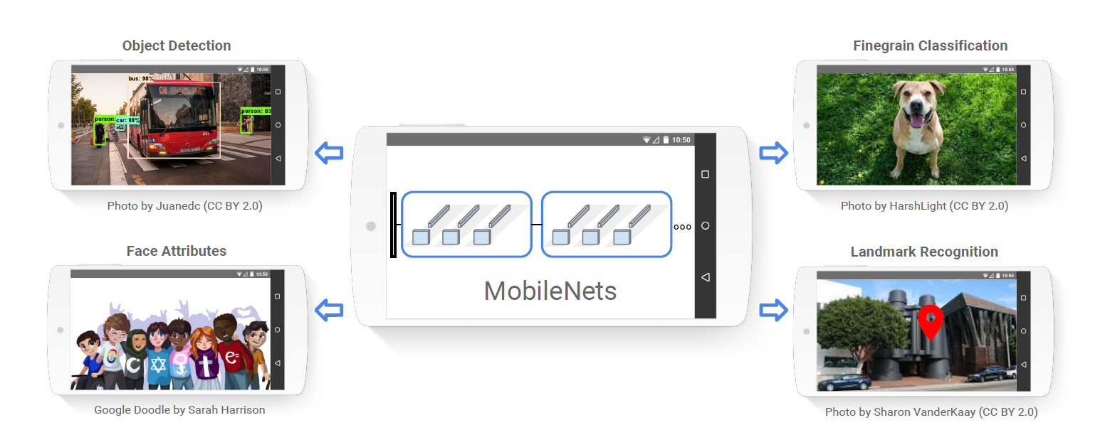
The motivation behind developing MobileNet arises from the growing usage of smartphones.  But, CNNs require significant computational resources and power, whereas smartphones have limited resources such as processing power, and power source.

Bringing real-time image processing into these devices would result in a new set of capabilities and functionalities. MobileNet, with the introduction of Depth-wise and Point-wise convolutions, reduced the limitation of these hardware resources.

Depthwise Separable Convolutions

Standard Convolutions

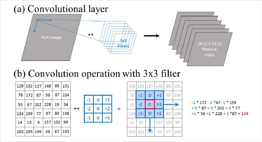
Convolution layers are the core of deep learning models. They extract features from an image. Here are the steps involved in a standard convolution operation:

• Defining the Filter (Kernel): A filter (also called a kernel) is a randomly initialized small matrix, that is used to detect features such as edges, textures, or patterns in images. The values of the matrix are updated during the training process through backpropagation.
• Sliding the Filter Across the Input: The filter is slid across the width and height of the image, at each step element-wise multiplication and summation operation is performed.
• Element-wise Multiplication and Summation: At each position, the result of the multiplication is then summed up to get a single number. This results in the formation of a feature map or an activation map. The output values (i.e., the sum) indicate the presence and strength of the feature detected by the filter.

However, this convolution operation has its limitations:

1. Higher Computational Cost: Due to the dense matrix multiplications (where each filter is convolved with all the input channels), it is computationally expensive. For example, if you have an input with 64 channels and apply 32 filters, each filter processes all 64 channels.
2. Increased Parameter Count: The number of parameters also grows significantly with an increase in the number of input and output channels. This is because each filter has to learn from all the input channels.

This growth in parameter counts and higher computational cost increases the memory usage and computation requirements to perform all these multiplications. This is a limiting factor for deployment in smartphones and IoT devices.

Depthwise convolution and Pointwise Convolution

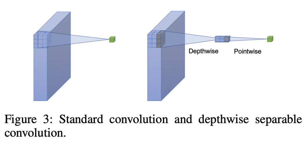
Depthwise Separable Convolution splits the standard convolution into two separate steps:

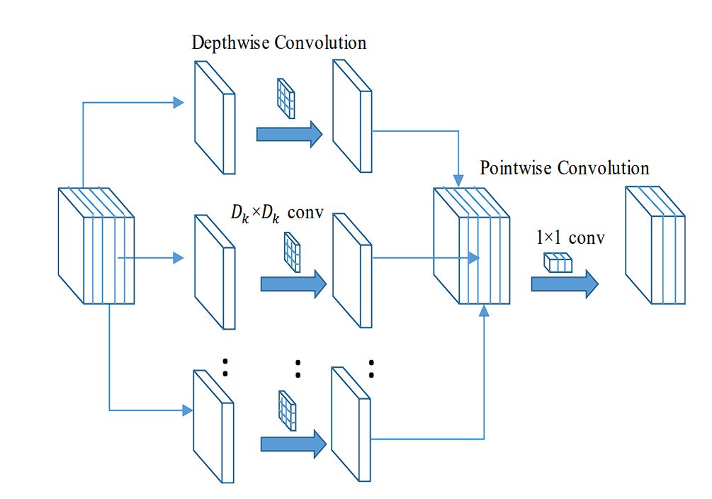
• Depthwise convolution: Applies a single filter to each input channel.
• Pointwise convolution (1×1 convolution): Combines the outputs from the depthwise convolution to create new features.

Steps in Depthwise Convolution

• Separation of Channels: Standard convolution applies filters to each channel of the input image. Whereas depthwise convolution only applies a single filter per input channel.
• Filter Application: As each filter is applied independently, the output is the result of convolving (multiplication and summation) a single input channel with a dedicated filter.
• Output Channels: The output of the depthwise convolution has the same number of channels as the input.
• Reduced Complexity: Compared to standard convolution, the total number of multiplicative operations is reduced.
• For standard convolution the total number of multiplicative operations = 𝐾×𝐾×𝐶×𝐷×height×width
• For depthwise convolution, the number of operations = 𝐾×𝐾×𝐶× height×width

Pointwise Convolution

To combine features or expand channels, the output of depthwise convolution is applied with pointwise convolution. This is a 1×1 filter, which is applied to each pixel. This combines or expands the channels.

1. Combining Channel Features: Depthwise convolution processes each input channel separately, therefore interaction between channels doesn’t happen. Pointwise convolution combines these independently processed channel features to create a new feature map. This allows the model to learn from the entire depth of feature maps.
2. Increases Model Capacity: The interactions between the channels increase the representational capacity of the network. The model can learn complex patterns that depend on the relationships between different feature channels.
3. Adjusting the Number of Channels: Pointwise convolution enables increasing or decreasing the number of channels in the output feature map.

MobileNet Architecture

The MobileNet architecture is built primarily using depthwise separable convolutions, with some exceptions like the first layer which uses a full convolution. This allows for efficient feature extraction.

Other layers like batch normalization and ReLU are included for activation. The model achieves down-sampling of the output feature from previous layers with stride convolutions.  At the end of the network, we have an average pooling layer, then a fully connected layer. The final layer is a SoftMax layer for classification. In total, MobileNet has 28 layers.

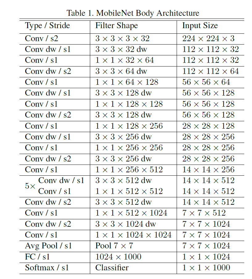
Moreover, the model heavily relies on the optimized 1×1 convolutions (MobileNet spends 95% of its computation time in 1×1 convolutions which also has 75% of the parameters). The convolution uses optimized general matrix multiply (GEMM) functions for efficiency.

The model is trained using RMSprop and asynchronous gradient descent. However, in comparison to training larger models, MobileNet training uses less regularization (such as weight decay), and data augmentation as smaller models are less prone to overfitting.

The model is quite small in size compared to various other models, however, MobileNet further uses two additional parameters to reduce model size and computation when it is necessary. These parameters are:

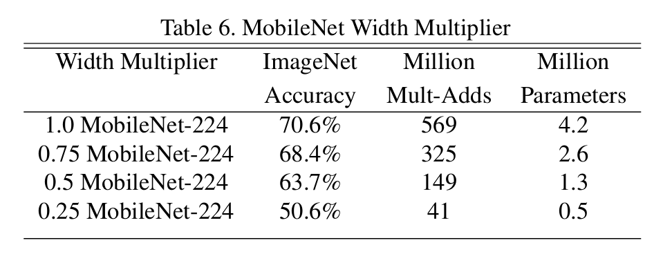
• Width Multiplier (α): The purpose of this parameter is to thin the network uniformly at each layer by α. Lower α values result in a smaller and faster model but with some accuracy trade-off.

  

• Resolution Multiplier (ρ): This is another hyperparameter for reducing computational cost. This reduces the input image resolution by the variable ρ. Lower ρ values lead to a smaller model but also decrease accuracy.

MobileNet Variants

MobileNet V2

Introduced by Google researchers in 2018, MobileNetV2 builds upon the ideas of the original MobileNet, enhancing its architecture to provide even better efficiency and accuracy.

Key Improvements

• Inverted Residuals: MobileNet v2 Introduced inverted residual blocks with bottlenecking. These blocks use linear bottlenecks between layers to reduce the number of channels processed, which further improves the efficiency. It also added short connections between these bottlenecks to improve information flow. Moreover, the last layer, which is usually a non-linear activation function (ReLU) is replaced by linear activation. As the data has a low spatial dimension in the bottleneck, linear activation performs better.

MobileNet V3

MobileNetV3 was released in 2019 with the following key features:

• Hardware-Aware NAS (Network Architecture Search) for Layer-wise Optimization: This technique utilizes an automated search process to find the best configuration design for mobile hardware. This works by exploring different network architectures evaluating their performance on mobile CPUs and then selecting the most efficient and accurate configuration.
• Squeeze-and-Excitation (SE) Modules: These modules analyze the feature maps produced by the convolutional layers and highlight the most important features.
• Hard Swish: This is an activation function designed for mobile processors. It offers a good balance between accuracy and computational efficiency and is less complex compared to ReLU.

Other Lightweight Models

• SqueezeNet: SqueezeNet is a similar model known for its small size, achieved by using 1×1 convolutions. SqueezeNet first compresses the data format and then expands it, by doing so, it removes the redundant features.
• ShuffleNet: ShuffleNet is another model designed for mobile devices. It utilizes pointwise group convolutions (by splitting feature channels into groups and applying convolutions independently within each group) and channel shuffle operations (this shuffles the order of channels after the group convolutions) to reduce computational costs.

Benchmarks and Performance

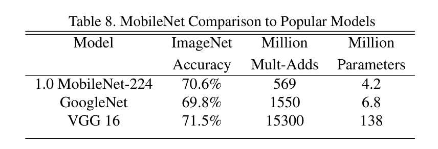
MobileNet has a significant advantage compared to models with standard convolutions, as it achieves similar high accuracy scores on the ImageNet dataset, but with substantially fewer parameters.

• It achieves accuracy close to VGG16 while being significantly smaller and less computationally expensive.
• It outperforms GoogLeNet in terms of accuracy with a smaller size and lower computational cost.

  

• MobileNet, when further decreased in size using width and resolution multiplier hyperparameter, outperformed AlexNet and SqueezeNet with its substantially efficient and smaller size.

Moreover, it outperformed various models that were significantly larger, on tasks such as:

• Fine-grained recognition (Stanford Dogs dataset)
• Large-scale geolocation (PlaNet)
• Face attribute classification (with knowledge distillation)
• Object detection (COCO dataset)
• Face embedding (distilled MobileNet from FaceNet)

Applications of MobileNet

Covid Detection

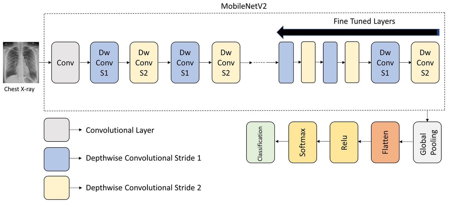
During the global pandemic due to Coronavirus, researchers developed a model using MobileNet to accurately classify chest X-ray images into three categories: normal, COVID-19, and viral pneumonia, with an accuracy of 99%.

Fish Detection

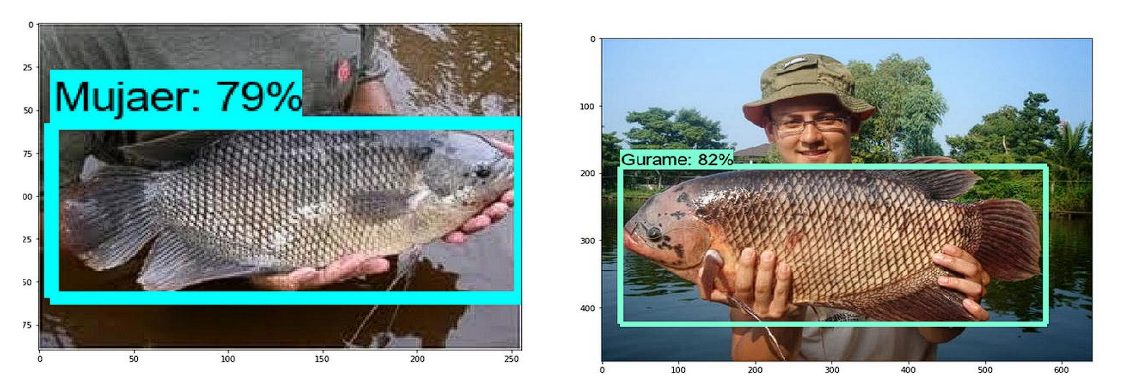
Freshwater fish farming is a profitable business that provides a source of income for over 60 million people, and accurately identifying fish species is crucial for the business.  Researchers used MobileNet V1 to train a model to classify freshwater fish from images. MobileNet was chosen because it could be run on the smartphone devices of the farmers. The resulting model achieved an accuracy rate of 90% in distinguishing between different types of fish.

Skin Cancer

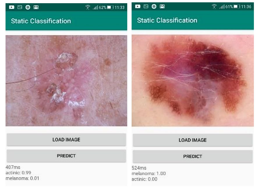
Mobile applications for detecting skin cancer are becoming popular. They all send the data to a server, and that server returns the result. However, this can’t be used in areas with poor Internet connectivity. As a result, researchers trained the MobileNet v2 model to detect and classify two types of skin cancer (Actinic Keratosis and Melanoma) in images using an Android device. The model achieved 90% accuracy, taking around 20 seconds.

Leaf Disease

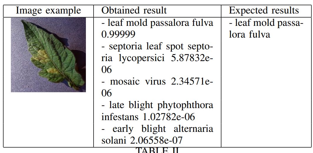
For a profitable tomato crop yield, early and accurate detection of tomato leaf diseases is crucial. Other CNN-based networks are large and require dedicated equipment. Researchers developed a mobile application that utilizes a MobileNet model to recognize 10 common tomato leaf diseases using a smartphone, achieving an accuracy of 90%.

Welding Defects

Welding defects can affect the quality and safety of welded structures and can result in accidents that can be life-threatening. X-ray imaging is used for inspecting welds for defects. Deep Learning models can be trained to detect defects, however, they require a large dataset. Researchers utilized transfer learning, which uses a pre-trained MobileNet model as a feature extractor, and then fine-tuned on welding defect X-ray images. The Transfer Learning-MobileNet model achieves a high classification accuracy of 97%, the performance is compared to other methods such as Xception, VGG-16, VGG-19, and ResNet-50, but with fewer resources.

Mask on face

Due to COVID-19, wearing masks in public was made mandatory in 2020, to prevent the spread of the virus.  Researchers trained the MobileNet model on roughly 9,000 images. The resulting model achieved an accuracy of 87.96% for detecting if a mask is worn and 93.5% for detecting if it’s worn correctly.

Conclusion

In this article, we looked at MobileNet, a highly efficient Neural Network model for mobile and embedded devices released by Google. It achieves its remarkable efficiency using depthwise separable convolution. Moreover, the model’s size can be further reduced by using width and resolution multiplier hyperparameters. With these advancements, MobileNet has made real-time image processing capabilities on mobile devices natively possible.

As a result, several mobile applications have been developed that can use the MobileNet model for image classification and object detection.