Convolution is a feature extractor in image processing that extracts key characteristics and attributes from images and outputs useful image representations.
CNNs learn features directly from the training data. These features can include edges, corners, textures, or other relevant attributes that aid in distinguishing an image and understanding its contents. Object detection and image classification models later use these extracted features.
Deep Learning extensively utilizes Convolutional Neural Networks (CNNs) in which convolution operations play a central role in automatic feature extraction. Traditional image processing relies on hand-crafted features, while CNNs revolutionize the process by autonomously learning optimal features directly from the training data.
What is Convolution?
Image processing utilizes convolution, a mathematical operation where a matrix (or kernel) traverses the image and performs a dot product with the overlapping region. A convolution operation involves the following steps:
- Define a small matrix (filter).
- This kernel moves across the input image.
- At each location, the convolution operation computes the dot product of the kernel and the portion of the image it overlaps.
- The result of each dot product forms a new matrix that represents transformed features of the original image.
The primary goal of using convolution in image processing is to extract important features from the image and discard the rest. This results in a condensed representation of an image.
How Convolution Works in CNNs
Convolution Neural Networks (CNNs) are a deep learning architectures that use multiple convolutional layers combined with multiple Neural Network Layers.
Each layer applies different filters (kernels) and captures various aspects of the image. With increasing layers, the features extracted become dense. The initial layers extract edges and texture, and the final layers extract parts of an image, for example, a head, eyes, or a tail.
Here is how convolution works in CNNs:
- Layers: Lower layers capture basic features, while deeper layers identify more complex patterns like parts of objects or entire objects.
- Learning Process: CNNs learn the filters during training. The network adjusts the filters to minimize the loss between the predicted and actual outcomes, thus optimizing the feature extraction process.
- Pooling Layers: After the convolution operations, pooling takes place, which reduces the spatial size of the representation. A pooling layer in CNN downsamples the spatial dimensions of the input feature maps and reduces their size while preserving important information.
- Activation Functions: Neural networks use activation functions, like ReLU (Rectified Linear Unit), at the end to introduce non-linearities. This helps the model learn more complex patterns.
A Convolution Operation
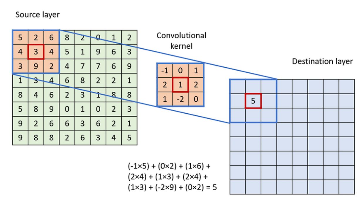
To apply the convolution:
- Overlay the Kernel on the Image: Start from the top-left corner of the image and place the kernel so that its center aligns with the current image pixel.
- Element-wise Multiplication: Multiply each element of the kernel with the corresponding element of the image it covers.
- Summation: Sum up all the products obtained from the element-wise multiplication. This sum forms a single pixel in the output feature map.
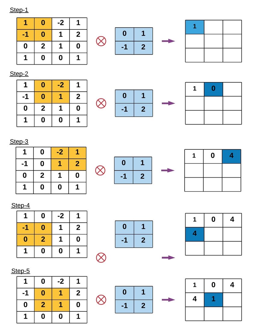
- Continue the Process: Slide the kernel over to the next pixel and repeat the process across the entire image.
Example of Convolution Operation
Key Terms in Convolution Operation
- Kernel Size: The convolution operation uses a filter, also known as a kernel, which is typically a square matrix. Common kernel sizes are 3×3, 5×5, or even larger. Larger kernels analyze more context within an image but come at the cost of reduced spatial resolution and increased computational demands.
- Stride: Stride is the number of pixels by which the kernel moves as it slides over the image. A stride of 1 means the kernel moves one pixel at a time, leading to a high-resolution output of the convolution. Increasing the stride reduces the output dimensions, which can help decrease computational cost and control overfitting but at the loss of some image detail.
- Padding: Padding involves adding an appropriate number of rows and columns (typically of zeros) to the input image borders. This ensures that the convolution kernel fits perfectly at the borders, allowing the output image to retain the same size as the input image, which is crucial for deep networks to allow the stacking of multiple layers.
Types of Convolution Operations
1D Convolution
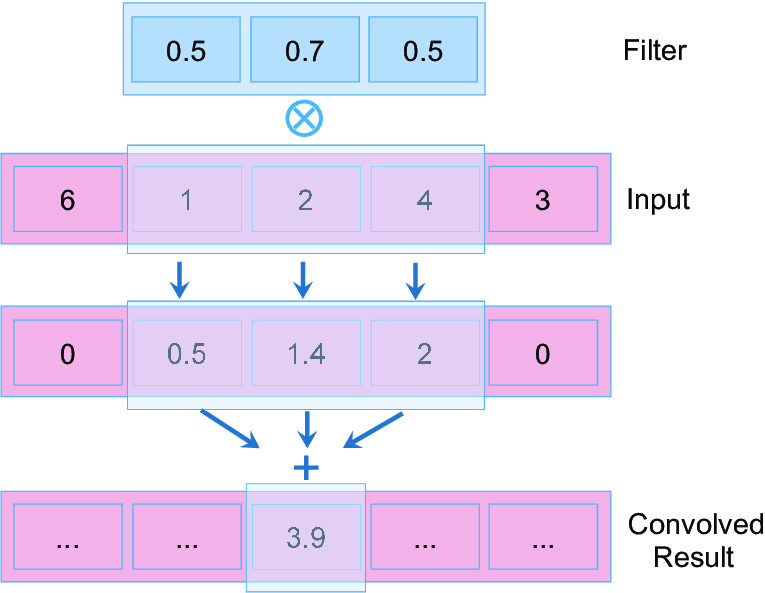
1D convolution is similar in principle to 2D convolution used in image processing.
In 1D convolution, a kernel or filter slides along the input data, performing element-wise multiplication followed by a sum, just as in 2D, but here the data and kernel are vectors instead of matrices.
Applications:
1D convolution can extract features from various kinds of sequential data, and is especially prevalent in:
- Audio Processing: For tasks such as speech recognition, sound classification, and music analysis, where it can help identify specific features of audio like pitch or tempo.

- Natural Language Processing (NLP): 1D convolutions can help in tasks such as sentiment analysis, topic classification, and even in generating text.
- Financial Time Series: For analyzing trends and patterns in financial markets, helping predict future movements based on past data.
- Sensor Data Analysis: Useful in analyzing sequences of sensor data in IoT applications, for anomaly detection or predictive maintenance.
3D Convolution
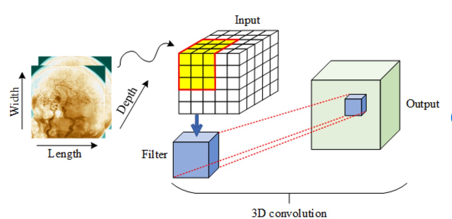
3D convolution extends the concept of 2D convolution by adding a dimension, which is useful for analyzing volumetric data.
Like 2D convolution, a three-dimensional kernel moves across the data, but it now simultaneously processes three axes (height, width, and depth).
Applications:
- AI Video Analytics: Processing video as volumetric data (width, height, time), where the temporal dimension (frames over time) can be treated similarly to spatial dimensions in images. The latest video generation model by OpenAI called Sora used 3D CNNs.
- Medical Imaging: Analyzing 3D scans, such as MRI or CT scans, where the additional dimension represents depth, providing more contextual information.
- Scientific Computing: Where volumetric data representations are common, such as in simulations of physical phenomena.
Dilated Convolution
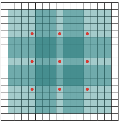
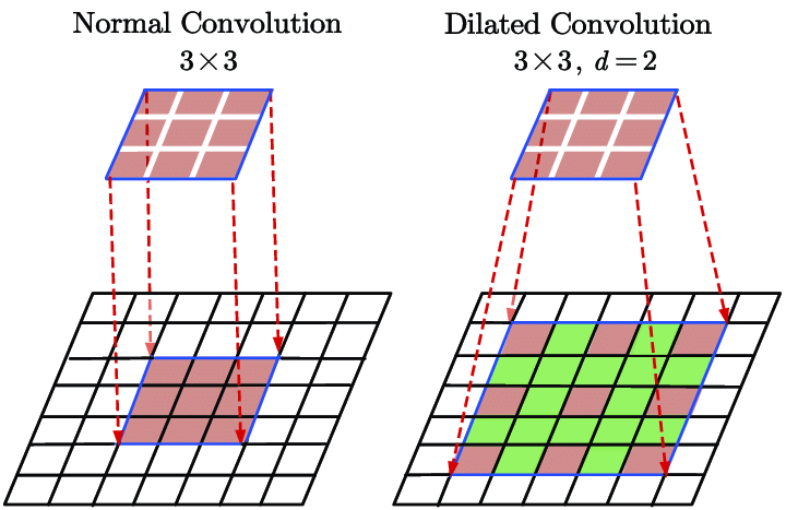
A variation of the standard convolution operation, dilated convolution expands the receptive field of the filter without significantly increasing the number of parameters. It achieves this by introducing gaps, or “dilations,” between the pixels in the convolution kernel.
In a dilated convolution, spaces are inserted between each element of the kernel to “spread out” the kernel. The l (dilation rate) controls the stride with which we sample the input data, expanding the kernel’s reach without adding more weights. For example, if d=2, there is one pixel skipped between each adjacent kernel element, making the kernel cover a larger area of the input.
Features
- Increased Receptive Field: Dilated convolution allows the receptive field of the network to grow exponentially with the depth of the network, rather than linearly. This is particularly useful in dense prediction tasks where contextual information from a larger area is beneficial for making accurate predictions at a pixel level.
- Preservation of Resolution: Unlike pooling layers, which reduce the spatial dimensions of the feature maps, dilated convolutions maintain the resolution of the input through the network layers. This characteristic is crucial for tasks where detailed spatial relationships need to be preserved, such as in pixel-level predictions.
- Efficiency: Dilated convolutions achieve these benefits without increasing the number of parameters, hence not increasing the model’s complexity or the computational cost as much as increasing the kernel size directly would.
Dilated Convolution is applied in various tasks of computer vision. Here are a few of those:
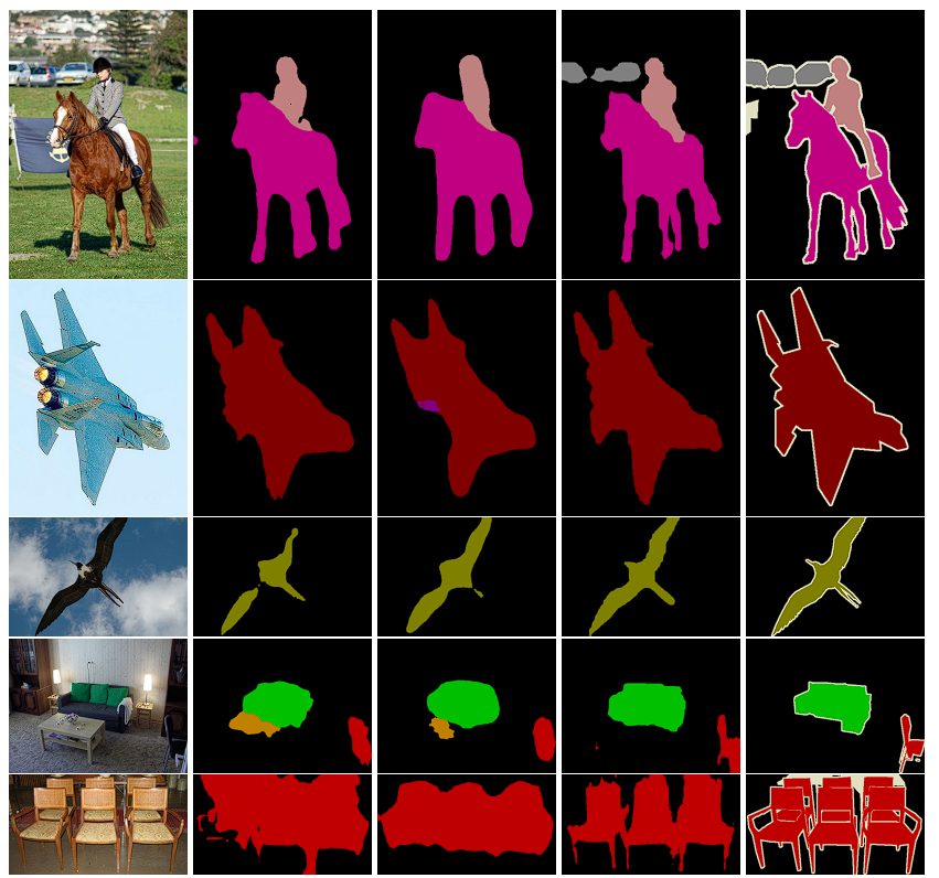
- Semantic Segmentation: In semantic segmentation, the goal is to assign a class label to each pixel in an image. Dilated convolutions are extensively used in segmentation models like DeepLab, where capturing broader context without losing detail is crucial. By using dilated convolutions, these models can efficiently enlarge their receptive fields to incorporate larger contexts, improving the accuracy of classifying each pixel.

Semantic Segmentation –source - Audio Processing: Dilated convolutions are also used in audio processing tasks, such as in WaveNet for generating raw audio. Here, dilations help capture information over longer audio sequences, which is essential when predicting subsequent audio samples.
- Video Processing: In video frame prediction and analysis, dilated convolutions help in understanding and leveraging the information over extended spatial and temporal contexts, which is beneficial for tasks like anomaly detection or future frame prediction.
Transposed Convolution
Transposed convolution is primarily used to increase the spatial dimensions of an input tensor. While standard convolution, by sliding a kernel over it produces a smaller output, a transposed convolution starts with the input, spreads it out (typically adding zeros in between elements, known as upsampling), and then applies a kernel to produce a larger output.
Standard convolutions typically extract features and reduce data dimensions, whereas transposed convolutions generate or expand data dimensions, such as generating higher-resolution images from lower-resolution ones. Instead of mapping multiple input pixels into one output pixel, transposed convolution maps one input pixel to multiple outputs.
Unlike standard convolution, where striding controls how far the filter jumps after each operation, in transposed convolution, the stride value represents the spacing between the inputs. For example, applying a filter with a stride of 2 to every second pixel in each dimension effectively doubles the dimensions of the output feature map if no padding is used.
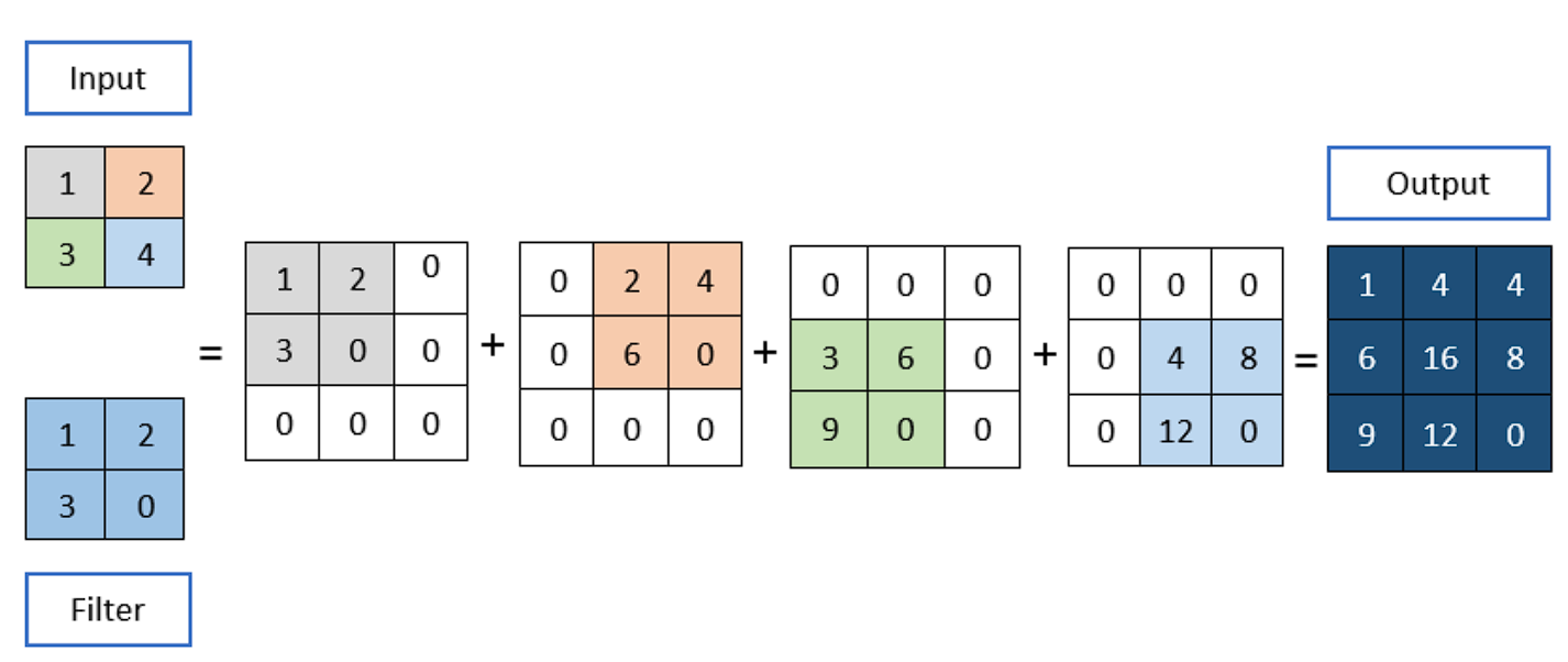
The generator component of Generative Adversarial Networks (GANs) and the decoder part of an AutoEncoder extensively use transposed convolutions.
In GANs, the generator starts with a random noise vector and applies several layers of transposed convolution to produce an output that has the same dimension as the desired data (e.g., generating a 64×64 image from a 100-dimensional noise vector). This process involves learning to upsample lower-dimensional feature representations to a full-resolution image.
Depthwise Separable Convolution
A depthwise convolution, an efficient form of convolution used to reduce computational cost and the number of parameters while maintaining similar performance, involves convolving each input channel with a different filter. The convolution takes place in two steps: Depthwise Convolution and then Pointwise Convolution. Here is how they work:
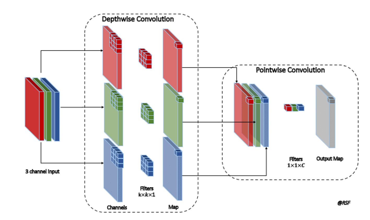
- Depthwise Convolution: A single convolutional filter applies separately to each channel of the input in depthwise convolution. A dedicated kernel convolves each channel. For instance, in an RGB image with 3 channels, each channel receives its kernel, ensuring that the output retains the same number of channels as the input.
- Pointwise Convolution: After depthwise convolution, pointwise convolution is applied. This step uses a 1×1 convolution to combine the outputs of the depthwise convolution across the channels. This means it takes the depthwise convolved channels and applies a 1×1 convolutional filter to each pixel, combining information across the different channels. Essentially, this step integrates the features extracted independently by the depthwise step, creating an aggregated feature map.
In standard convolutions, the number of parameters quickly escalates with increases in input depth and output channels due to the full connection between input and output channels. Depthwise separable convolutions separate this process, drastically reducing the number of parameters by focusing first on spatial features independently per channel and then combining these features linearly.
For example, if we have the following:
- Input Feature Map: 32 Channels
- Output Feature Map: 64 Channels
- Kernel Size for Convolution: 3 x 3
Standard Convolution:
- Parameters =3×3×32×64
- Total Parameters =18432
Depthwise Separable Convolution:
- Depthwise Convolution:
- Parameters= 3 x 3 x 32
- Parameters=288
- Pointwise Convolution:
- Parameteres= 1 x 1 x32 x 64
- Parameters= 2048
- Total Prameters= 2336
Applications in Mobile and Edge Computing
Depthwise separable convolutions are particularly prominent in models designed for mobile and edge computing, like the MobileNet architectures. These models are optimized for environments where computational resources, power, and memory are limited:
- MobileNet Architectures: MobileNet models utilize depthwise separable convolutions extensively to provide lightweight deep neural networks. These models maintain high accuracy while being computationally efficient and small in size, making them suitable for running on mobile devices, embedded systems, or any platform where resources are constrained.
- Suitability for Real-Time Applications: The efficiency of depthwise separable convolutions makes them ideal for real-time applications on mobile devices, such as real-time image and video processing, face detection, and AR and VR.
Deformable Convolution
Deformable convolution is an advanced convolution operation that introduces learnable parameters to adjust the spatial sampling locations in the input feature map. This adaptability allows the convolutional grid to deform based on the input, making the convolution operation more flexible and better suited to handle variations in the input data.
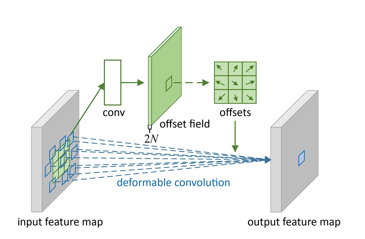
In traditional convolution, the filter applies over a fixed grid in the input feature map. However, deformable convolution adds an offset to each spatial sampling location in the grid, learned during the training process.
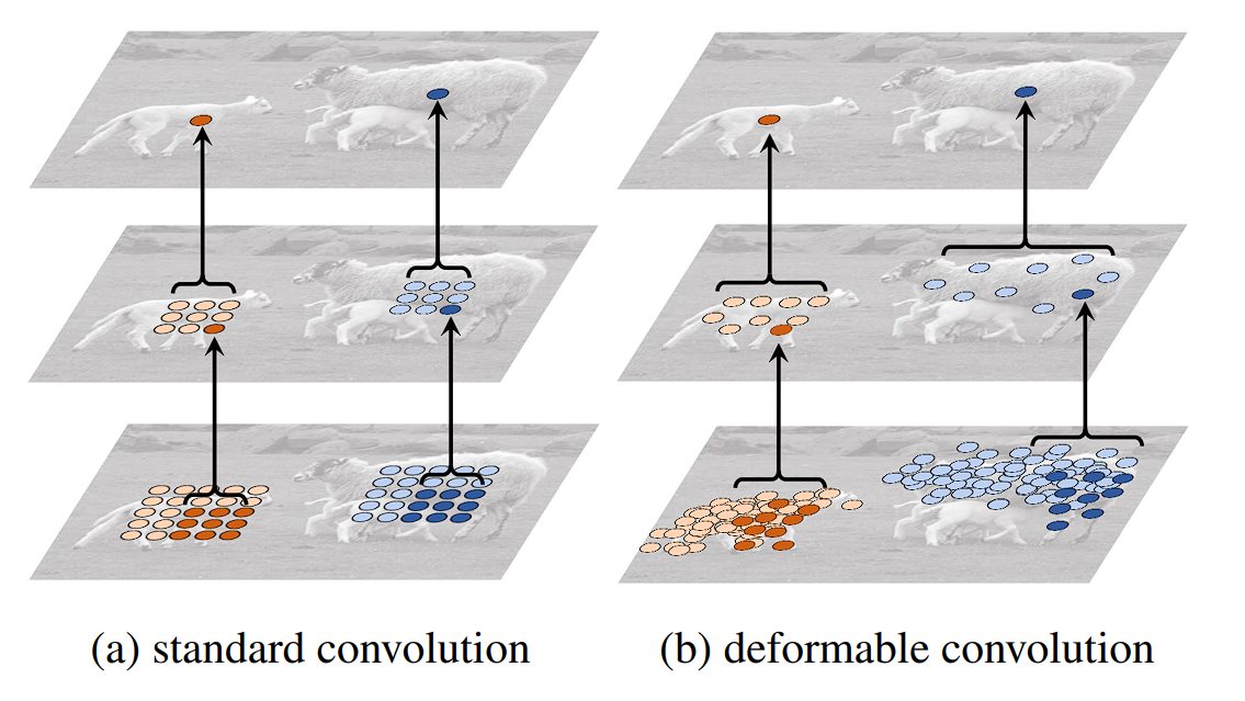
These offsets allow the convolutional filter to adapt its shape and size dynamically, focusing more effectively on relevant features by deforming around them. Additional convolutional layers designed to predict the best deformation for each specific input learn the offsets.
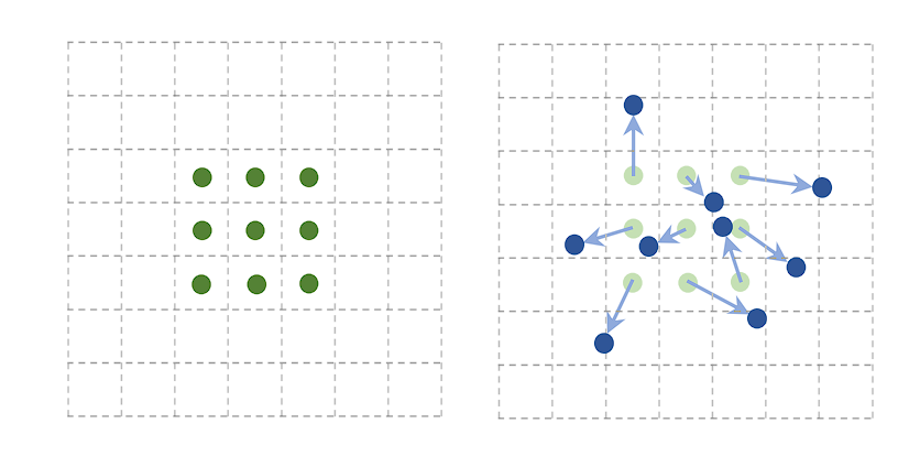
Deformable convolutions have been successfully integrated into several state-of-the-art object detection frameworks, such as Faster R-CNN and YOLO, providing improvements in detecting objects with non-rigid transformations and complex orientations. Here are its applications:
- Image Recognition: It is beneficial in cases where objects can appear in different sizes, shapes, or orientations.
- Video Analysis: Deformable convolutions can adapt to movements and changes in posture, angle, or scale within video frames, enhancing the ability of models to track and analyze objects dynamically.
- Enhancing Model Robustness: By allowing the convolutional operation to adapt to the data, deformable convolutions can increase the robustness of models against variations in the appearance of objects, leading to more accurate predictions across a wider range of conditions.
Recap and What’s Next
In this blog, we went from standard convolution operations to various specialized convolutions. However, Convolution is a fundamental operation in image processing used to extract features from images. These features are essential for tasks like image recognition and classification. Standard convolutions involve manipulating image data with a small matrix (kernel) to achieve this. The size, stride, and padding of the kernel all influence the outcome.
Beyond standard convolutions, the specialized types like dilated, transposed, and depthwise separable convolutions are each designed for specific purposes. These variants address challenges such as computational efficiency and handling complex data. Several real-world object detection models are powered by these diverse convolution operations.
As research in this area of artificial intelligence (AI) and machine learning continues, new convolutional techniques will further enhance our ability to analyze and utilize imagery.
To learn about more aspects of the worlds of machine learning and computer vision, check out the following articles:
