Neural Radiance Fields (NeRFs): A Technical Exploration

Neural Radiance Fields (NeRFs) are a deep learning technique that uses fully connected neural networks to represent 3D scenes from a collection of 2D images and then render them to synthesize novel views. With their ability to synthesize realistic new viewpoints, Neural Radiance Fields excel in a wide range of 3D capture scenarios, from panoramic views of enclosed spaces to vast, open landscapes.

Recall your last vacation where you captured a few photos of your favorite place. NeRFs offer the potential to revisit such scenes in immersive 3D, generating realistic views from multiple angles.

This article will explore how those neural radiance fields work, their variations, optimization, applications, and more.

Let’s get started!

Understanding NeRFs: Neural Radiance Fields Explained

Synthesizing novel views from images has always been a core challenge in computer vision and computer graphics, with various methods developed over the years. Neural Radiance Fields (NeRFs) have emerged as an innovative solution, attracting significant attention for their ability to learn complex scene representations. At their core, many NeRF methods utilize Multilayer Perceptron (MLP) neural networks to create those complex scene representations.

Let’s briefly explore MLPs.

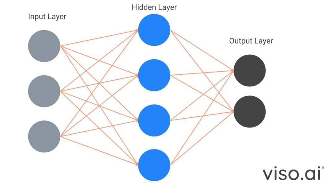
MLPs are a class of feedforward neural networks consisting of fully connected layers of nodes. They excel at feature extraction and encoding spatial relationships, often used for representing geometric 3D shapes or image data. They achieve this through positional encoding, which transforms coordinates into representations that capture details at varying scales.

NeRFs build upon this by utilizing an optimized MLP architecture to create scene representations in a way suitable for realistic 3D scene synthesis. This representation combined with rendering methods creates the final 3D scene. The original NeRF method focuses on learning a scene representation and then leverages the volume rendering method to synthesize realistic 3D images.

Let’s get into both the scene representation and rendering aspects of NeRFs, starting with how they represent scenes.

Scene Representation

Neural Radiance Fields represent continuous scenes mathematically as a vector-valued function with five dimensions.

An optimized MLP network with no convolutional layers takes 3D coordinates (x, y, z) plus a 2D viewing direction (θ, φ) as input creating the 5D vector, and outputs density (σ) which is the transparency and color (r, g, b) values. This mapping is learned in the training process.

Here we can see the inputs and outputs for NeRFs.

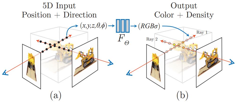
To synthesize novel views, NeRFs sample 5D coordinates along multiple camera rays and feed these into an optimized MLP network to produce color and volume density values. While many NeRF variations exist, a baseline NeRF architecture often uses a simple but optimized MLP network.

Let’s examine this core design.

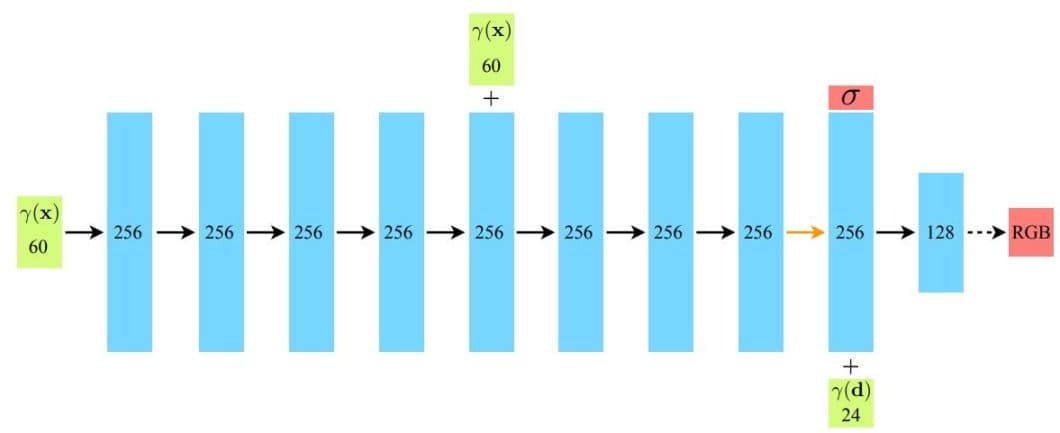
1. First, the input 3D coordinates (x) undergo positional encoding (γ(x)) to capture fine details. This encoded information flows through 8 hidden layers (Blue), each employing ReLU activations (Black arrows).
2. A skip connection at the 5th layer improves information flow and potentially speeds up training by concatenating (“+”) the input to the layer activation.
3. The network so far produces two outputs, volume density (indicated by σ), which stands for opacity values across the scene surface, and a 256-dimensional feature vector that contributes to accurate color predictions.
4. Finally, the feature vector is combined with a positionally encoded viewing direction (γ(d)) and passed to one additional layer with 128 channels.
5. The final layer with sigmoid activation (dotted arrow) calculates the emitted RGB radiance at position (x) along a ray direction (d).

Now that we have the scene representation as RGB and volume density values, the next step is to use rendering methods to synthesize the 3D scene from any view.

Volume Rendering

Rendering is the process of synthesizing an image from a scene file containing feature information using a certain function or equation, neural radiance fields often achieve this using volume rendering methods. Imagine the NeRF-captured scene as a 3D grid of tiny cubes called voxels. Each voxel holds the color (RGB) and density (σ) values that the NeRF has learned during training.

To render a view, we must first define a camera position from which we cast rays through this voxel grid. Along each ray, the algorithm samples multiple 3D points. Then the NeRF neural network provides color (RGB) and density (σ) values for each sample point.

Here is a visual showing the rays and the information extracted from each passing ray.

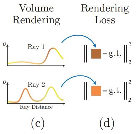
Classic volume rendering equations then combine this information to composite the samples into the final image based on the camera position relative to the volume. Also, as seen in the visual we can use rendering loss to minimize the difference between the rendered and ground truth images during optimization. The beauty of neural radiance fields is that the scene representation is view-dependent, meaning the scene representation differs based on the viewing angle.

Here is an example.

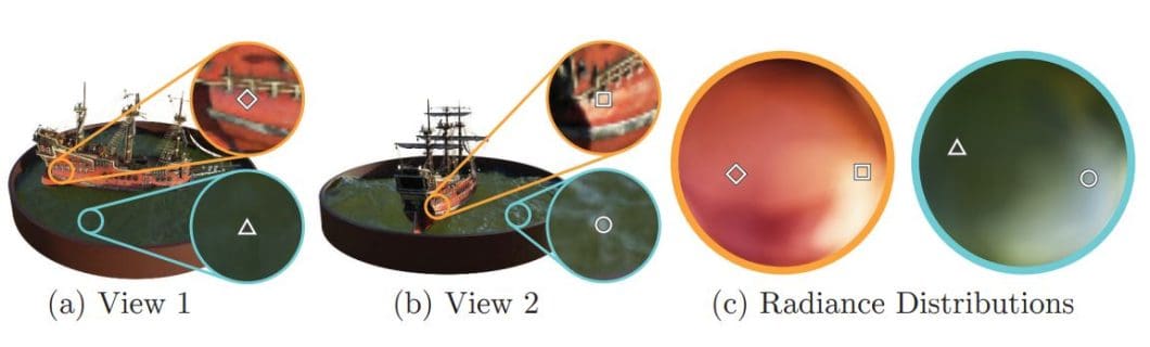
This demonstrates how two fixed 3D points appear differently when viewed from two distinct camera positions.

A camera position can be one of the following:

• Fixed: Camera line of sight is preset.
• Tracking: The camera moves based on preset movements in a video scene.
• Interactive: The camera position can be changed interactively and the NeRF would predict the changes.

Let’s now explore optimization methods in NeRFs for better image synthesis.

Optimization of Neural Radiance Fields: Methods and Techniques

Previously, we explored the core components of neural radiance fields, from scene representation to rendering novel views from those representations. However, without careful optimization, those steps would produce low-quality images and be too slow for practical use or real-time use cases. Optimization methods differ across NeRF variants. Here, we will list some key techniques that set the stage for NeRFs to reach state-of-the-art performance.

Positional Encoding

Using positional encoding with neural radiance fields was a true milestone for view synthesis as it provided big performance enhancement in the quality and details of the output.

Positional encoding is simple, before passing the 3D coordinates to the MLP we transform them into a higher-dimensional space using a set of carefully chosen functions. This transformation helps the network understand the spatial relationships within the scene, allowing it to represent complex details more effectively.

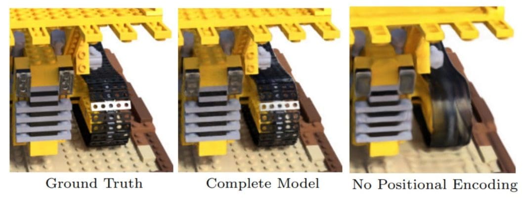
Even though other optimization methods were used in the complete model, positional encoding has proven essential for the quality of the output. This method is also used within Transformers but for a different goal. In NLP, positional encoding is used to give a hint about the order of words.

Hierarchical Volume Sampling

While positional encoding enhances the representation in Neural Radiance Fields, hierarchical volume sampling optimizes volume rendering. NeRFs sample multiple points along camera rays to render an image, but many of these samples end up in empty space or occluded areas, contributing little to the final image. Hierarchical volume sampling addresses this problem for faster, more effective rendering.

The principle is that, instead of treating the entire scene uniformly, this method adopts a two-stage sampling approach known as Coarse-Fine Networks (CFN):

• Coarse Sampling: A first pass provides a rough estimate of where features like surfaces or denser areas are likely located.
• Fine Sampling: Focuses computational effort on these relevant regions, providing the fine details needed for a high-quality image.

The two main benefits of this technique are:

• Speed: Hierarchical volume sampling speeds up rendering without reducing image quality by allocating more samples to important areas.
• Efficiency: This technique avoids wasting computational resources on empty or occluded regions of the scene.

Other Methods

Neural Radiance Field optimization continues to advance, as researchers develop new and innovative techniques. Here is a brief overview of a few additional methods that show promise for enhancing Neural Radiance Fields.

1. Scene Representation Enhancements: While the original NeRF used a simple MLP, other NeRF variations might have specialized architectures that lead to better quality output, and more efficiency.
2. Advanced Sampling Strategies: Other sampling techniques that build on hierarchical volume sampling exist, focusing rendering efforts on areas most likely to impact the final image, proving useful for efficiency and detailing.
3. Regularization: Methods to prevent overfitting of the training data, encourage NeRF models to generalize to new viewpoints more reliably.
4. Optimized Loss Functions: Optimized loss functions teach the NeRF to bring the output closer to ground truth making more visually realistic images.

The variety of optimization methods in NeRFs opens the door for many exciting variations. Let’s explore some significant NeRFs in the next section.

Types of Neural Radiance Fields

Since its introduction, Neural Radiance Fields have seen rapid innovation. Researchers have developed many NeRF variations, each building upon existing techniques but addressing challenges and unlocking new possibilities.

The original NeRF provided a good foundation but had limitations in speed, performance, efficiency, and adaptability, which the following variants offered advancements in. This section will explore some significant NeRF variations, highlighting their unique strengths and contributions.

Mip-NeRF

The original NeRF performed well when representing scenes viewed from distances similar to its training data, but produced blurry or aliased images when dealing with details across different scales.

Mip-NeRF addresses this limitation by extending NeRF to represent the scene across a continuous range of scales. To achieve this, instead of casting single rays per pixel, Mip-NeRF uses conical frustums, geometrical shapes resembling cone-shaped beams inspired by MipMapping.

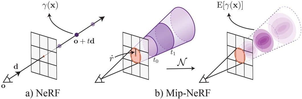
Importantly, Mip-NeRF achieves these visual improvements while also being 7% faster than the original NeRF and reducing model size by half. This is achieved through a key technique called Integrated Positional Encoding (IPE), which extends NeRF’s encoding to represent regions of space rather than just single points.

pixelNeRF

pixelNeRF made a great advancement in Neural Radiance Fields, as the original NeRF had limitations when dealing with scenarios involving few input images, as it required extensive per-scene optimization. This made it impractical for scenarios with limited input views.

The solution proposed by pixelNeRF aimed to overcome this limitation, offering impressive novel view synthesis from just one or a few images. This advancement in generalization is achieved by training PixelNeRF across multiple scenes, allowing it to learn a scene prior.

This includes a key architectural change: using a fully convolutional architecture. PixelNeRF first extracts a feature grid from the input image(s). Then it samples features from this grid via projection and interpolation for each query point and viewing direction.

These spatially aligned image features condition the NeRF, guiding the prediction of density and color.

The architecture of pixelNeRF provides many advantages for better novel view synthesis. Once trained, PixelNeRF predicts NeRF representations in a feed-forward manner, eliminating the need for time-consuming per-scene optimization.

Other advantages include:

• No 3D Supervision: It can be trained directly on multi-view image datasets.
• Camera-Centric: It predicts NeRFs in the camera coordinate frame of the input, making it adaptable to diverse scenes.
• Spatial Alignment: The convolutional design preserves the spatial relationship between the image and the 3D representation.

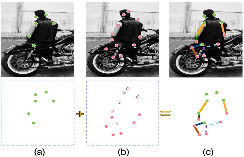
Here are some results from the pixelNeRF paper.

Mega-NeRF:

Another big advancement in Neural Radiance Fields is MegaNerf. While Mip-NeRF and pixelNeRF address image quality and data efficiency,  Mega-NeRF explores the representation and synthesis of large-scale real-world environments. Mega-NeRF enables the creation and interactive exploration of 3D scenes encompassing entire buildings or city blocks captured by drones.

This leap in scale depends on two key innovations:

• Sparse Network Structure: Mega-NeRF recognizes that most image data only contributes to a limited portion of the scene. So it employs a sparse network with specialized parameters for specific regions, significantly improving efficiency and model capacity.
• Geometric Clustering: This approach uses a simple geometric clustering algorithm that partitions training data (pixels) into distinct NeRF submodules that can be trained in parallel.

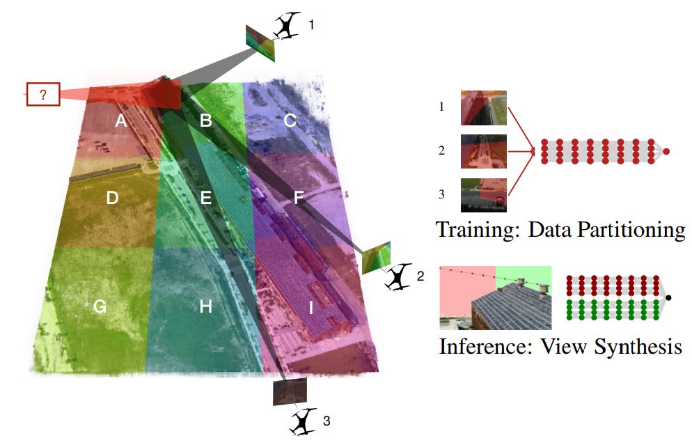
While other models like Kilo-NeRF achieved similar large-scale performance, Mega-Nerf is much larger, faster, and more precise. Another feature of Mega-Nerf is temporal coherence for rendering which allows for smooth, interactive fly-throughs of these massive environments by caching occupancy and color information from previous views.

Researchers are constantly exploring diverse approaches fitting NeRFs to different use case scenarios, innovative variations like GANeRF uses concepts from GAN networks to enhance view synthesis, and Light Field Neural Rendering which uses transformers. This ongoing development unlocks the vast potential of Neural Radiance Fields for a wide range of applications.

Applications of Neural Radiance Fields: Use Cases and Code

Neural Radiance Fields have exploded in popularity since their introduction and with good reason. The ability of a neural radiance field to capture and represent real-world scenes has led to many applications across various domains.

Let’s delve into some of the most interesting use cases that showcase the power of NeRFs.

1. Product Visualization: NeRF’s ability to represent fine details enables the creation of photorealistic product renders, revolutionizing e-commerce and marketing materials. Users can examine products from every angle in exceptional detail.
2. Digital Archiving: Museums and historical societies can use NeRFs to capture artifacts with unprecedented detail, preserving them digitally for future generations.
3. 3D Content Creation from Photos: Individuals can turn personal photo collections into 3D models. This opens possibilities for personalized digital environments and assets for social media or AR experiences.
4. Virtual Tourism and Exploration: Users can explore landmarks and remote locations built from minimal image sets.
5. Urban Planning and Simulation: Realistic urban simulations, aid in architectural design, transportation planning, and disaster response training.
6. VR Environments: Create expansive, highly detailed, and realistic VR worlds without the size limitations of traditional 3D modeling.
7. Robotic Navigation and Perception: Provide robots with highly realistic scene representations, improving their ability to navigate and interact with complex environments.
8. Synthetic Data: Nerf’s ability to synthesize novel views with fast rendering can be used to generate highly realistic synthetic data.

Code

We have explored a lot of ground with Neural Radiance Fields – the concepts, the variations, and the potential applications. But NeRFs aren’t exactly an easy model to run. They need more setup, and each variation is different depending on the use case.

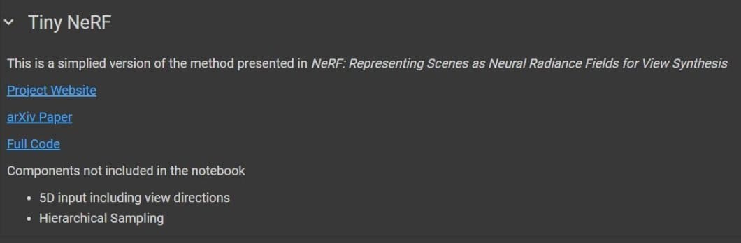
For now, we will explore a simplified implementation called Tiny NeRF on Colab. This will give you a taste of NeRF coding. You can find the notebook here. When you open the notebook, you will see a quick intro to what Tiny NeRF is and other useful links.

Before running the first block, which prepares the environment and imports needed libraries, make sure to delete this line of code:

if IN_COLAB:
    %tensorflow_version 1.x

Or change it to:

if IN_COLAB:
    %tensorflow_version 2.x

Either way, it’s the same because Colab will only use Tensorflow version 2 and higher.

In the next block of code, we will be importing the data, Colab will not allow you to get this data unless you add “–no-check-certificate” Here is how it should look:

if not os.path.exists('tiny_nerf_data.npz'):
    !wget http://cseweb.ucsd.edu/~viscomp/projects/LF/papers/ECCV20/nerf/tiny_nerf_data.npz --no-check-certificate

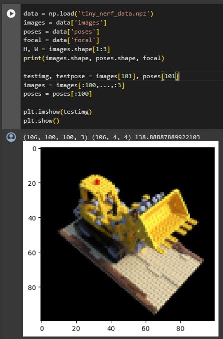
Now that we have the data, the next cell should load it and show an example from it.

Then you can run the 2 cells under the “Optimize NeRF” section of the notebook. This will likely take around 12 minutes, but it is interesting to see how the Neural Radiance Field improves in rendering the scene. You can also test to increase the iterations, but no improvements will be made.

The next code cell will allow for interactive visualization with the rendered scene.

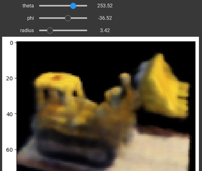
Adjusting the values will allow you to see different viewpoints. Note that it can be very slow in showing the changes. Lastly, you can render and view a video of the 3D scene in the next blocks.

What’s Next?

From its original form to the specialized variations we have explored, the journey of Neural Radiance Fields highlights its incredible flexibility. Whether photorealistic product renders, immersive virtual experiences, or enhanced robotics, NeRFs are reshaping how we interact with the digital world.

As researchers continue to push boundaries, we can anticipate even more applications and advancements. The future of NeRFs is undoubtedly bright, promising a world where 3D representation and digital interaction will reach great heights.