Xception, short for Extreme Inception, is a Deep Learning model developed by Francois Chollet at Google, continuing the popularity of Inception architecture, and further perfecting it.
The inception architecture utilizes inception modules, however, the Xception model replaces it with depthwise separable convolution layers, which totals 36 layers. When we compare the Xception model with the Inception V3 model, it only slightly performs better on the ImageNet dataset, however, on larger datasets consisting of 350 million images, Xception performs significantly better.
The Journey of Deep Learning Models in Computer Vision
Utilization of deep learning architectures in computer vision began with AlexNet in 2012, It was the first to use Convolutional Neural Network architectures (CNNs) for image recognition, which won the ImageNet Large Scale Visual Recognition Challenge (ILSVRC).
After AlexNet, the trend was to increase the convolutional blocks’ depth in the models, leading to researchers creating very deep models such as ZFNet, VGGNet, and GoogLeNet (inception v1 model).
These models experimented with various techniques and combinations to improve accuracy and efficiency, with techniques such as smaller convolutional filters, deeper layers, and inception modules.
The Inception Model
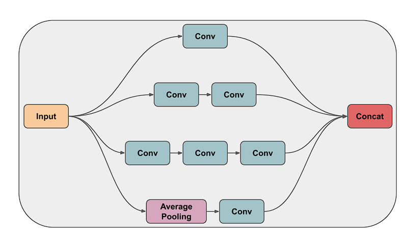
A standard convolution layer tries to learn filters in a 3D space, namely: width, height (spatial correlation), and channels (cross-channel correlation), thereby utilizing a single kernel to learn them.
However, the Inception module divides the task of spatial and cross-channel correlation using filters of different sizes (1×1, 3×3, 5×5) in parallel, hence, benchmarks proved that this is an efficient and better way to learn filters.
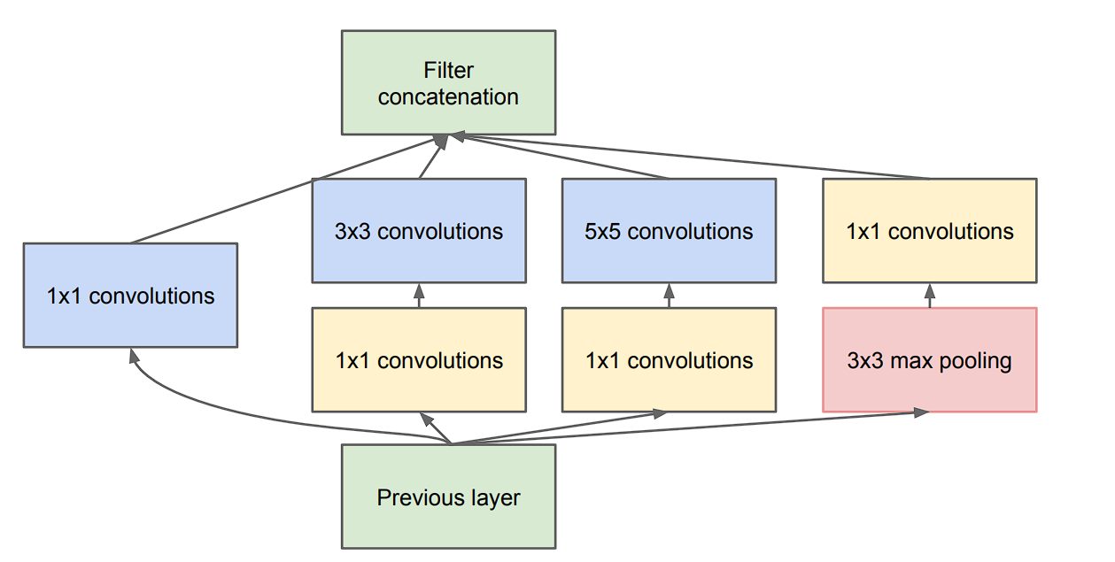
Xception takes an even more aggressive approach as it entirely decouples the task of cross-channel and spatial correlation. This gave it the name Extreme Inception Model.
Xception Architecture
The Xception model’s core is made up of depthwise separable convolutions. Therefore, before diving into individual components of Xception’s architecture, let’s take a look at depthwise separable convolution.
Depthwise Separable Convolution
Standard convolution learns filters in 3D space, with each kernel learning width, height, and channels.
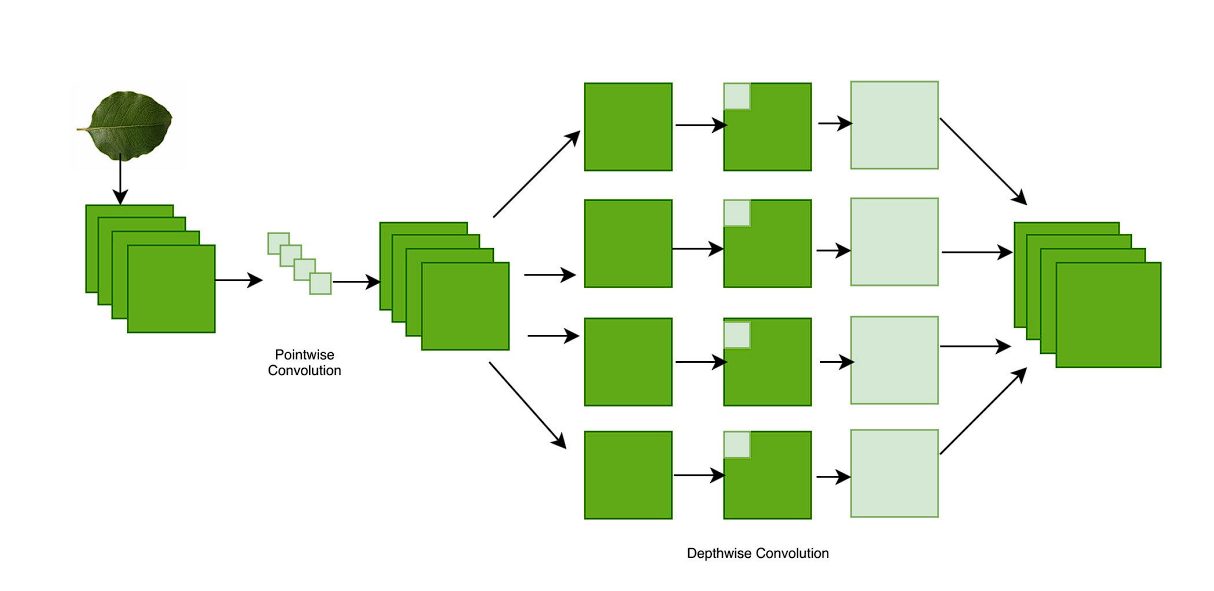
Whereas, a depthwise separable convolution divides the process into two distinctive processes using depth-wise convolution and pointwise convolution:
- Depthwise Convolution: Here, a single filter is applied to each input channel separately. For example, if an image has three color channels (red, green, and blue), a separate filter is applied to each color channel.
- Pointwise Convolution: After the depthwise convolution, a pointwise convolution is applied. This is a 1×1 filter that combines the output of the depthwise convolution into a single feature map.
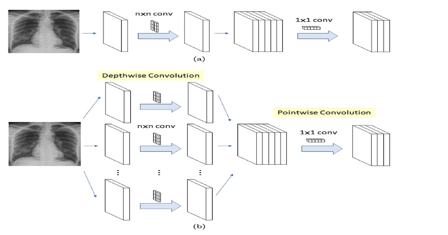
Xception utilizes a slightly modified version of this. In the original depthwise separable convolution, we first perform depthwise convolution and then pointwise convolution. The Xception model performs pointwise convolution first (1×1), and then the depthwise convolution using various nxn filters.
The Three Parts of Xception Architecture
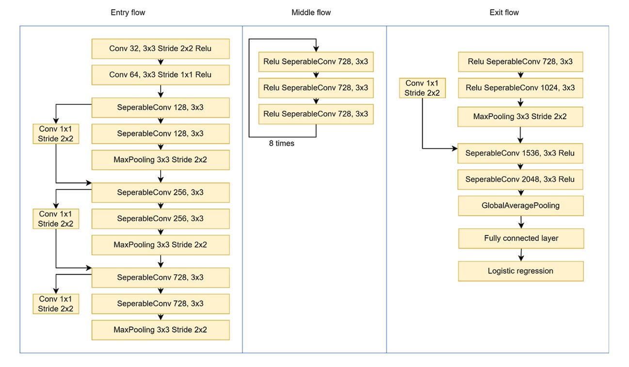
We divide the entire Xception architecture into three main parts: the entry flow, the middle flow, and the exit flow, with skip connections around the 36 layers.
- Entry Flow
- The input image is 299×299 pixels with 3 channels (RGB).
- A 3×3 convolution layer is used with 32 filters and a stride of 2×2. This reduces the image size and extracts low-level features. To introduce non-linearity, the ReLU activation function is applied.
- It is followed by another 3×3 convolution layer with 64 filters and ReLU.
- After the initial low-level feature extraction, the modified depthwise separable convolution layer is applied, along with the 1×1 convolution layer. Max pooling (3×3 with stride=2) reduces the size of the feature map.
- Middle Flow
- This block is repeated eight times.
- Each repetition consists of:
- Depthwise separable convolution with 728 filters and a 3×3 kernel.
- ReLU activation.
- By repeating it eight times, the middle flow progressively extracts higher-level features from the image.
- Exit Flow
- Separable convolution with 728, 1024, 1536, and 2048 filters, all with 3×3 kernels, further extracts complex features.
- Global Average Pooling summarizes the entire feature map into a single vector.
- Finally, at the end, a fully connected layer with logistic regression classifies the images.
Regularization Techniques
Deep learning models aim to generalize (the model’s ability to adapt properly to new, previously unseen data), whereas overfitting stops the model from generalizing.
Overfitting is when a model learns noise from the training data or overly learns the training data. Regularization techniques help to prevent overfitting in machine learning models. The Xception model uses weight decay and dropout regularization techniques.
Weight Decay
Weight decay, also called L2 regularization, works by adding penalties to the larger weights. This helps to keep the size of weights small (when the weights are small, each feature contributes less to the overall decision of the model, which makes the model less sensitive to fluctuations in input data).
Without weight decay, the weight could grow exponentially, leading to overfitting.
Dropout
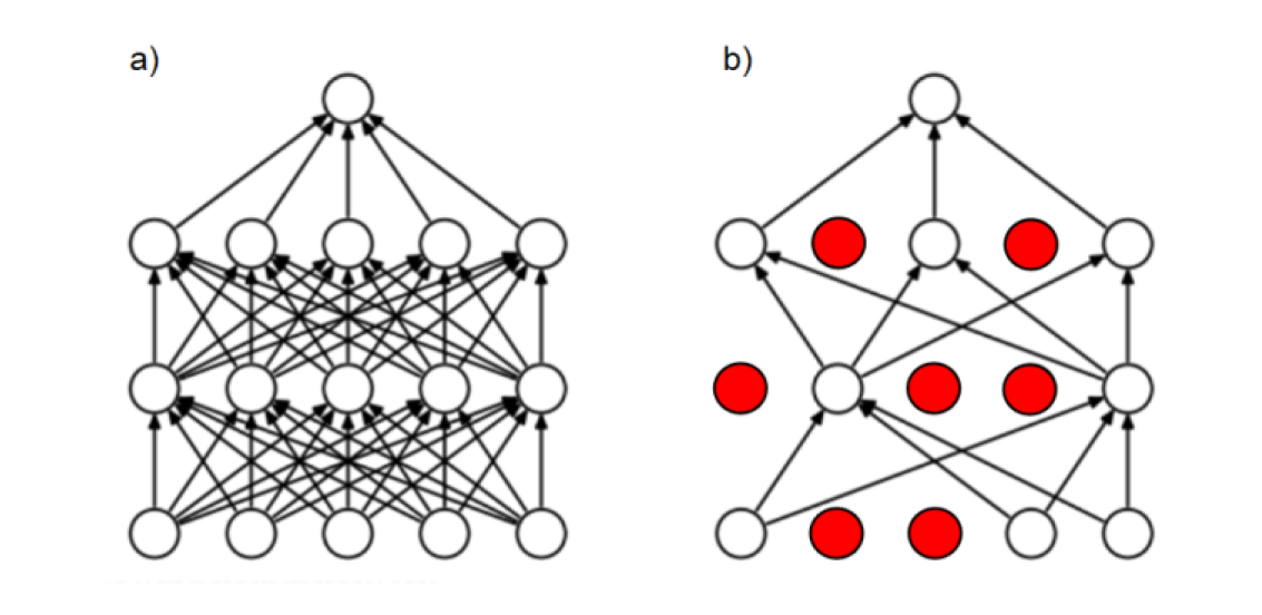
This regularization technique works by randomly ignoring certain neurons in training, during forward and backward passes. The dropout rate controls the probability that a certain neuron will be dropped. As a result, for each training batch, a different subset of neurons is activated, leading to more robust learning.
Residual Connections
The Xception model has several skip connections throughout its architecture.
When training a very Deep Neural Network, the gradients used during training to update weights become small and even sometimes vanish. This is a major problem all deep learning models face. To overcome this, researchers came up with residual connections in their paper in 2016 on the ResNet model.
Residual connections, also called skip connections, work by providing a connection between the earlier layers in the network with deeper or final layers in the network. These connections help the flow of gradients without vanishing, as they bypass the intermediate layers.
When using residual learning, the layers learn to approximate the difference (or residual) between the input and the output, as a result, the original function 𝐻(𝑥) becomes 𝐻(𝑥)=𝐹(𝑥)+𝑥
Benefits of Residual Connections:
- Deeper Networks: Enables training of much deeper networks
- Improved Gradient Flow: By providing a direct path for gradients to flow back to earlier layers, we solve the vanishing gradient problem.
- Better Performance
Today, ResNet is a standard component in deep learning architectures.
Performance and Benchmarks
The original paper on the Xception model used two different datasets: ImageNet and JFT. ImageNet is a popular dataset, which consists of 15 million labeled images with 20,000 categories. Testing used a subset of ImageNet containing around 1.2 million training images and 1,000 categories.
JFT is a large dataset that consists of over 350 million high-resolution images annotated with labels of 17,000 classes.
We compare the Xception model with Inception v3 due to a similar parameter count. This ensures that any performance difference between the two models is a result of architecture efficiency and not its size.
The result obtained for ImageNet showed a marginal difference between the two models, however with a larger dataset like JFT, the Xception model shows a 4.3% relative improvement. Moreover, the Xception model outperforms the ResNet-152 and VGG-16 models.
Applications of the Xception Model
Plan Identification
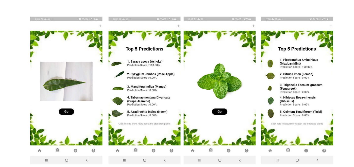
Researchers developed the DeepHerb application, a system for automatically identifying medicinal plants using deep learning techniques. The DeepHerb dataset includes 2515 leaf images from 40 species of Indian herbs.
The researchers used various pre-trained convolutional neural network (CNN) architectures like VGG16, VGG19, InceptionV3, and Xception. The best-performing model was the Xception model which achieved an accuracy of 97.5%. The mobile application, HerbSnap, provided herb identification with a 1-second prediction time.
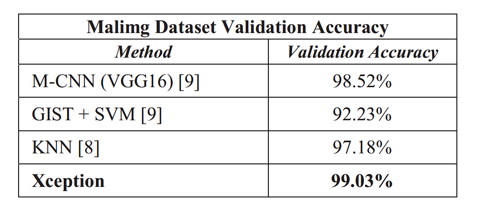
Malware Detection
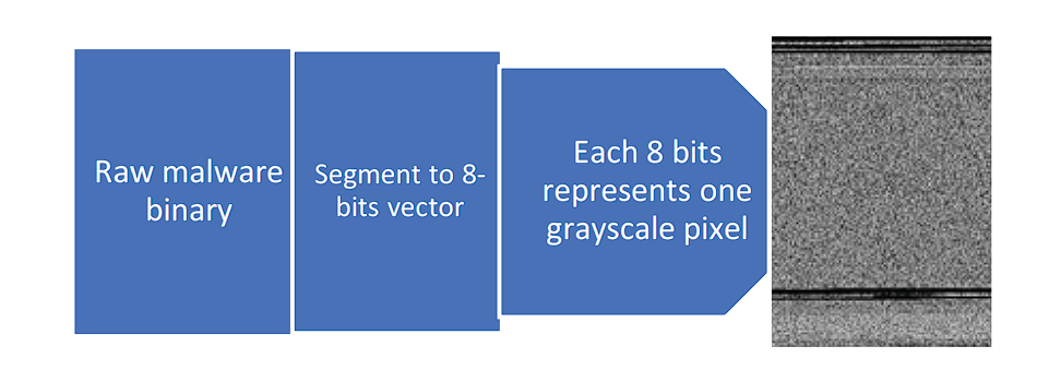
Researchers utilized the Xception Network for malware classification using transfer learning. They first converted malware files into grayscale images and then classified them using a pre-trained Xception model fine-tuned for malware detection. Two datasets were used for this task: the Malimg Dataset (9,339 malware grayscale images, 25 malware families) and the Microsoft Malware Dataset (10,868 malware grayscale images, 10,873 testing samples, 9 malware families)
The resulting Xception model achieved an accuracy (99.04% on Malimg, 99.17% on Microsoft) compared to other methods such as VGG16.
The researchers also further improved the accuracy by creating an Ensemble Model that combined the prediction results from two types of malware files (.asm and .bytes). The resulting Ensemble Model achieved an accuracy of 99.94%.
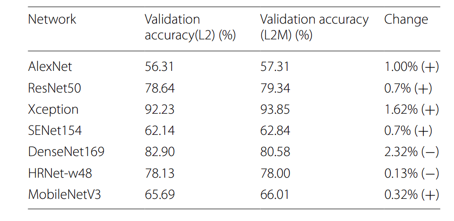
Leaf Disease Detection
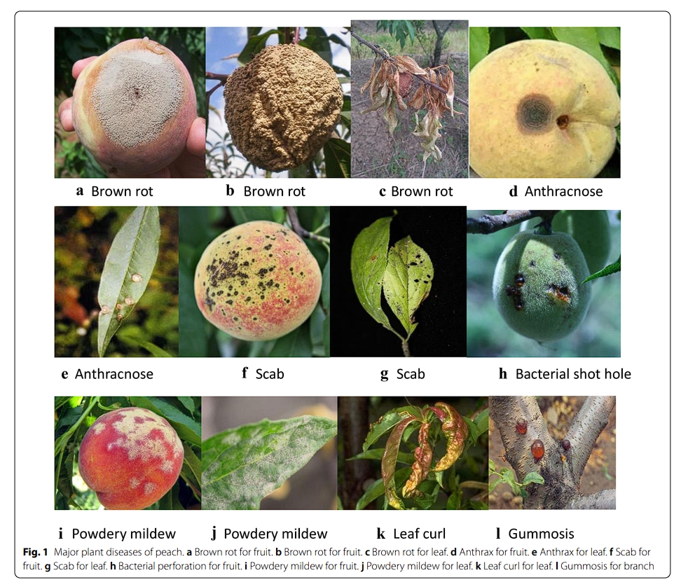
A study analyzed different diseases found in peache and their classifications using different deep-learning models. The deep learning models consisted of MobileNet, ResNet, AlexNet, and more. Amongst all these models, the Xception model with L2M regularization achieved the highest score of 93.85%, making it the most effective model in that study for peach disease classification.
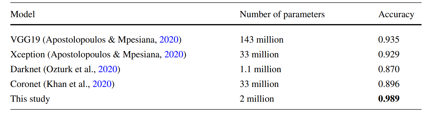
COVID-19 Detection
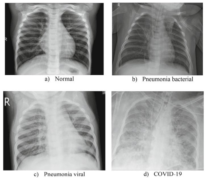
Researchers developed an improved Xception-based model using genetic algorithm techniques for network optimization. The resulting Xception model achieved high accuracy results on the X-Ray images—99.6% for two cass scores and 98.9% for three classes, significantly outperforming other deep learning (such as DenseNet169, HRNet-w48, and AlexNet) used in the study.
What’s Next With the Xception Model?
In this blog, we looked at the Xception model, a model that improved upon the popular Inception model released by Google. The key improvement made in the Xception model was the use of depthwise separable convolution. This saw significant improvement on large datasets such as JFT, however, there was an insignificant difference on smaller datasets such as ImageNet.
However, this showed that depthwise separable convolution was better than the inception module. Several researchers proved it by modifying the original Xception model to gain a significant advantage in accuracy over previous models. Moreover, after the Xception model, MobileNets released later also utilized depthwise convolution for a light deep learning model, capable of running on mobile phones.
Learn more about AI and computer vision models:
- The Ultimate Guide to AI Models
- A Rundown of the Best Lightweight Computer Vision Models
- A Typical Workflow of How to Build a Machine Learning Model
- Modern AI Development and Foundation Models
- Exploring Multi-modal AI with Vision-Language Models