Semantic segmentation is a computer vision task that involves classifying each pixel in an image into a predefined category. Unlike object detection, which identifies objects and draws bounding boxes around them, semantic segmentation labels each pixel in the image, deciding if it belongs to a certain category.
Semantic segmentation has significant importance in various fields, for example, in autonomous driving it helps understand and interpret the surroundings by identifying the area covered by roads, pedestrians, traffic vehicles, and other objects. In medical fields, it helps segment different anatomical structures (e.g., organs, tissues, tumors) in medical scans, and in agriculture, it is used for monitoring crops, detecting diseases, and managing resources by analyzing aerial or satellite images.
In this blog, we will look into the architecture of a popular image segmentation model called DeepLab. But before doing so, we will overview how image segmentation is performed.
About us: Viso.ai provides the leading end-to-end Computer Vision Platform Viso Suite. Global organizations use it to develop, deploy, and scale all computer vision applications in one place, with automated infrastructure. Get a personal demo.
How is Semantic Segmentation Performed?
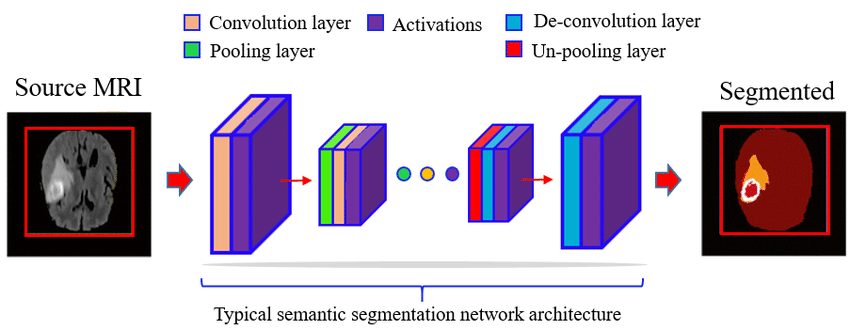
Semantic segmentation involves the following steps:
- Large datasets of images with pixel-level annotations (labels) are collected and then used for training the segmentation models.
- Common deep learning architectures include Fully Convolutional Networks (FCNs), U-Net, SegNet, and DeepLab.
- During the training phase, the model learns to predict the class of a single pixel. The model first classifies and localizes a certain object in the image. Then the pixels in the image are classified into different categories.
- Then during inference, the trained model predicts the class of each pixel in new, unseen images.
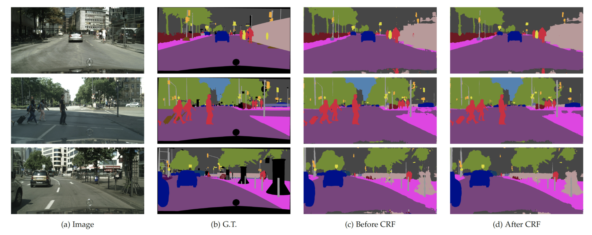
- Several post-processing techniques are used including coloring of the image, which is usually seen. Other techniques like Conditional Random Fields (CRFs) are used to refine the segmentation results to make the boundaries smoother and more accurate.
What is DeepLab Network?

DeepLab is a family of semantic segmentation models developed by Google Research and is known for its ability to capture fine-grained details and perform semantic segmentation on high-resolution images.
This model has several versions, each improving upon the previous one. However, the core architecture of DeepLab remains the same.
DeepLab v1
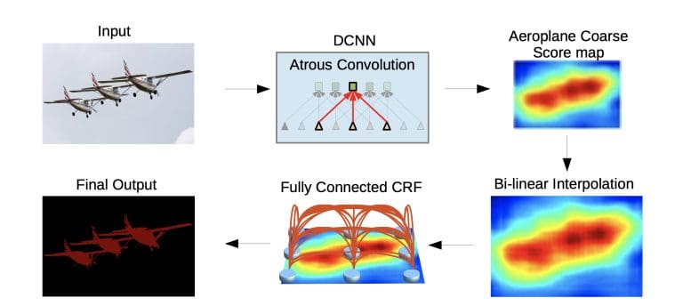
DeepLab introduces several key innovations for image segmentation, but one of the most important is the use of Atrous convolution (Dilated Convolution).
Deep Convolutional Neural Network (DCNN):
DeepLab architecture uses the VGG-16 deep Convolutional Neural Network as its feature extractor, providing strong representation and capturing high-level features for accurate segmentation.
However, DeepLab v1 replaces the final fully connected layers in VGG-16 with convolutional layers and utilizes atrous convolutions. These convolutions allow the network to capture features at multiple scales without losing spatial resolution, which is crucial for accurate segmentation.
What is Atrous Convolution?
Atrous convolutions are modified versions of standard convolutions, here the filter is modified to increase the receptive field of the network. However, increasing the receptive field usually results in an increased number of parameters.
However, in atrous separable convolution, an increase in the receptive field happens without the increase in the number of parameters or losing resolution, helping in capturing multi-scale contextual information.
How Does Atrous Convolution Work?
Here’s how atrous convolution works:
- In a standard convolution, the filter is applied to the input feature map.
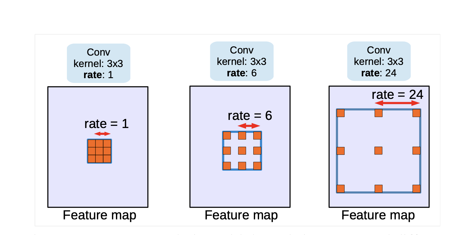
- In an atrous convolution, the filter is applied with gaps (or holes) between the filter elements, which are specified by the dilation rate.
The dilation rate (denoted as r) controls the spacing between the values in the filter. A dilation rate of 1 corresponds to a standard convolution, and a higher value than 1 creates a gap in the filter.
By increasing the dilation rate, the receptive field of the convolution expands without increasing the number of parameters or the computation cost.
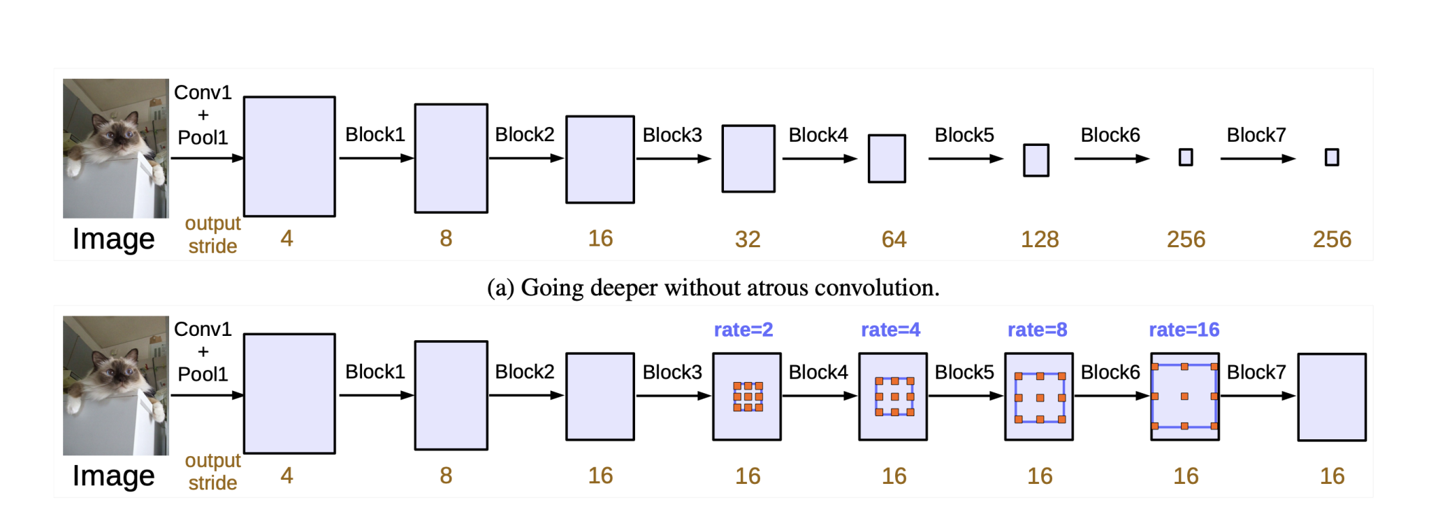
One might assume that the gaps could lead to missing important features. However, in practice, the gaps allow the network to capture multi-scale context efficiently. This is particularly useful for tasks like semantic segmentation where understanding the context around a pixel is crucial.
Moreover, in the later versions of DeepLab, we can find Atrous convolutions combined with other convolutional layers (both standard and atrous) in a network. This combination ensures that features captured at different scales and resolutions are integrated, mitigating any potential issues from sparse sampling.
CRF Based Post-processing
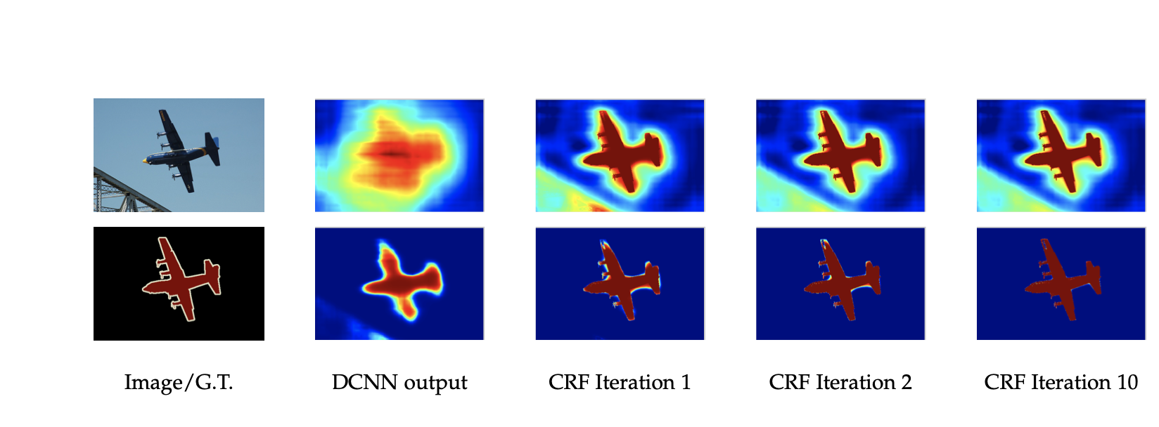
After semantic segmentation is done, DeepLab uses CRF post-processing to refine the segmentation. Conditional Random Field (CRF) works as a post-processing step, helping to sharpen object boundaries and improve the spatial coherence of the segmentation output. Here is how it works:
- The DCNN in DeepLab predicts a probability for each pixel that belongs to a specific class. This generates a preliminary segmentation mask.
- The CRF takes this initial segmentation and the image itself as inputs. It considers the relationships between neighboring pixels and their predicted labels. Then the CRF calculates two types of probabilities:
- Unary Potentials: These represent the initial class probabilities predicted by the DCNN for each pixel.
- Pairwise Potentials: These capture the relationships between neighboring pixels. They encourage pixels with similar features or spatial proximity to have the same label.
By considering both these probabilities, the CRF refines the initial segmentation probabilities.
DeepLab v2
DeepLabv2 introduced several significant enhancements and changes over its DeepLabv1.
The key changes in DeepLabv2 include:
1. Atrous Spatial Pyramid Pooling (ASPP)
One of the most notable changes is the introduction of the Atrous Spatial Pyramid Pooling (ASPP) module.
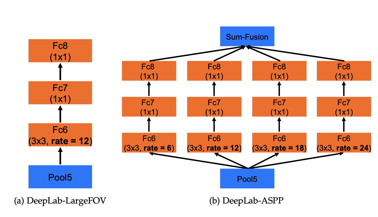
ASPP applies atrous convolution with different dilation rates in parallel. This allows it to capture multi-scale information effectively, making the model handle objects at various scales and capture global context more effectively.
As the DeepLabv1 relied solely on atrous convolutions, they capture information at a particular scale only depending upon the dilation rate, however, they miss very small or very large objects in an image.
To overcome this limitation, DeepLabv2 introduced ASPP (which uses multiple atrous convolutions with different strides aligned in parallel). Here is how It works:
- The input feature map is fed into several atrous convolution layers, each with a different dilation rate.
- Each convolution with a specific rate captures information at a different scale. A lower rate focuses on capturing finer details (smaller objects), while a higher rate captures information over a larger area (larger objects).
- In the end, the outputs from all these atrous convolutions are concatenated. This combined output incorporates features from various scales, making the network better able to understand objects of different sizes within the image.
2. DenseCRF
DeepLabv2 improves the CRF-based post-processing step by using a DenseCRF, which more accurately refines the segmentation boundaries, as it uses both pixel-level and higher-order potentials to enhance the spatial consistency and object boundary delineation in the segmentation output.
Standard CRFs can be applied to various tasks that are not related to computer vision. In contrast, DenseCRF is specifically designed for image segmentation, where all pixels are considered neighbors in a fully connected graph. This allows it to capture the spatial relationships between all pixels and their predicted labels.
3. Deeper Backbone Networks
While DeepLabv1 uses architectures like VGG-16, DeepLabv2 incorporates deeper and more powerful backbone networks such as ResNet-101. These deeper networks provide better feature representations, contributing to more accurate segmentation results.
4. Training with MS-COCO
DeepLabv2 includes training on the MS-COCO dataset in addition to the PASCAL VOC dataset, helping the model to generalize better and perform on diverse and complex scenarios.
DeepLab v3
DeepLabv3 further improves upon DeepLab v2, enhancing the performance and accuracy of semantic segmentation. The main changes in DeepLabv3 include:
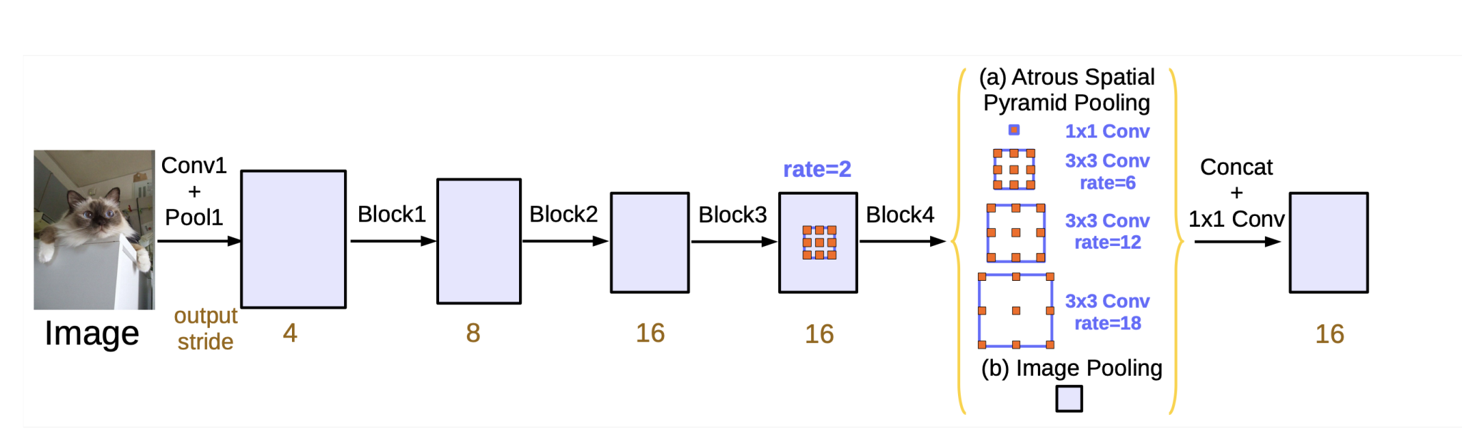
1. Enhanced Atrous Spatial Pyramid Pooling (ASPP)
DeepLabv3 refines the ASPP module by incorporating batch normalization and using both global average pooling with the already introduced, atrous convolution with multiple dilation rates.
2. Deeper and More Powerful Backbone Networks
DeepLabv3 uses even deeper and more powerful backbone networks, such as ResNet, and the more computationally efficient Xception architecture. These backbones offer improved feature extraction capabilities, which contribute to better segmentation performance.
3. No Explicit Decoder
Although encoder-decoder architecture is quite common in segmentation tasks, DeepLabv3 achieves excellent performance using a simpler design without a specific decoder stage. The ASPP and feature extraction layers provide sufficient performance to capture and process information.
4. Global Pooling
The ASPP module in DeepLabv3 includes global average pooling, which captures global context information and helps the model understand the broader scene layout. This operation takes the entire feature map generated by the backbone network and squeezes it into a single vector.
This is performed to capture image-level features, as these represent the overall context of the image, summarizing the entire image and scene. This is crucial for DeepLab semantic image segmentation, as it helps the model understand the relationships between different objects in the image.
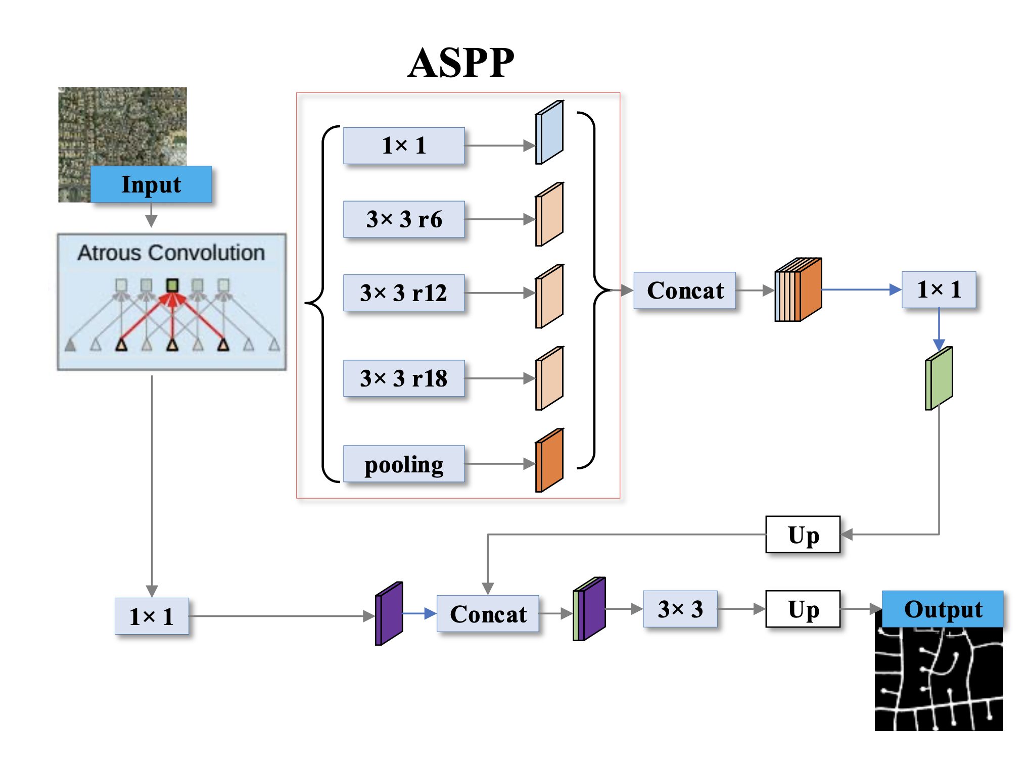
5. 1×1 Convolution
DeepLabv3 also introduces 1×1 convolution. In regular convolutions, the filter has a size larger than 1×1. This filter slides across the input image, performing element-wise multiplication and summation with the overlapping region of the image to generate a new feature map.
A 1×1 convolution, however, uses a filter of size 1×1. This means it considers only a single pixel at a time from the input feature map.
While this might seem like a simple operation that doesn’t capture much information, however, 1×1 convolutions offer several advantages:
- Dimensionality Reduction: A key benefit is the ability to reduce the number of channels in the output feature map. By applying a 1×1 convolution with a specific number of output channels, the model can compress the information from a larger number of input channels. This helps control model complexity and potentially reduce overfitting during training.
- Feature Learning: The 1×1 convolution acts as a feature transformation layer, making the model learn a more compact and informative representation of the image-level features. It can emphasize the most relevant aspects of the global context for the segmentation task.
This is how global average pooling and 1×1 convolution are used in deepLabv3:
- DeepLabv3 first performs global average pooling on the final feature map from the backbone.
- The resulting image-level features are then passed through a 1×1 convolution.
- This processed version of the image-level features is then concatenated with the outputs from atrous convolutions with different dilation rates (another component of ASPP).
- The combined features provide a rich representation that incorporates both local details captured by atrous convolutions and global context captured by the processed image-level features.
Conclusion
In this blog, we looked at the DeepLab neural network series and the significant advancements made in the field of image segmentation.
DeepLab image segmentation model laid the foundation with the introduction of atrous convolution, which allowed for capturing multi-scale context without increasing computation. Moreover, It employed a CRF for post-processing to refine segmentation boundaries.
The DeepLabv2 Improved upon DeepLabv1 by introducing the Atrous Spatial Pyramid Pooling (ASPP) module, which allowed for multi-scale context aggregation. Moreover, the use of deeper backbone networks and training on larger datasets like MS-COCO contributed to better performance. The DenseCRF refinement step improved spatial coherence and boundary accuracy.
The third version, DeepLabv3, further refined the ASPP module by incorporating batch normalization and global average pooling for even better multi-scale feature extraction and context understanding. DeepLabv3 uses even deeper and more efficient backbone networks like the Xception network.
To learn more about computer vision, we suggest checking out our other blogs:
- What are Liquid Neural Networks?
- Introduction to Spatial Transformer Networks
- Capsule Networks: A New Approach to Deep Learning
- Deep Belief Networks (DBNs) Explained
- Guide to Generative Adversarial Networks (GANs)