In this article, we will discuss the branch of machine learning that is semi-supervised learning by going over the underlying scenario, unique approaches to semi-supervised learning, and the assumptions needed to operate in such scenarios effectively. Afterward, we will investigate several semi-supervised learning algorithms, such as the generative Gaussian mixture algorithm, self-training, and co-training.
What is Semi-supervised Learning?
Semi-supervised learning is a branch of machine learning that attempts to solve problems that require or include both labeled and unlabeled data to train AI models. This employs concepts of mathematics, such as characteristics of both clustering and classification methods.
Semi-supervised learning is an employable method due to the high availability of unlabeled samples and the caveats of labeling large datasets with the utmost accuracy. Furthermore, semi-supervised learning methods allow extending contextual information given by labeled samples to a larger unlabeled dataset without significant accuracy loss.
We recommend checking out our article about supervised and unsupervised learning, which is the basis for semi-supervised learning.
When to use Semi-supervised Machine Learning?
Semi-supervised machine learning is useful in a variety of scenarios (Computer Vision, Natural Language Processing, etc.) where any amount of labeled data is scarce or expensive to obtain. For example, in medical imaging, manually annotating a large dataset can be time-consuming and costly. In such cases, using a smaller set of labeled data in combination with a larger set of unlabeled data can lead to improved model performance compared to using only labeled data.
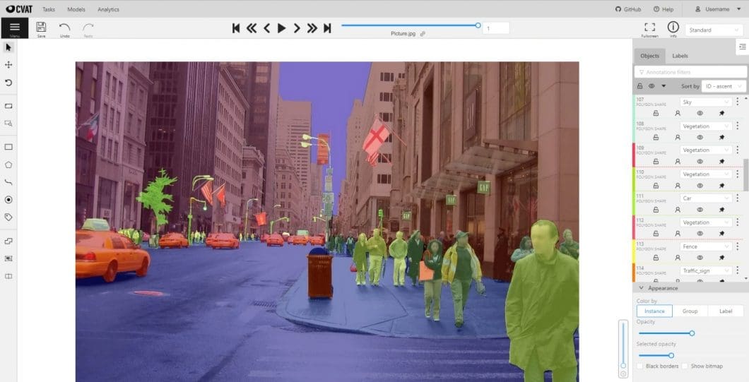
Additionally, semi-supervised learning can be beneficial when the task at hand requires a large amount of data to train a model with high accuracy. This is because it allows the model to learn from a larger amount of data, even if not all of it is labeled.
Here are popular use cases of semi-supervised machine learning:
- Image Classification: When the task is to classify images into different classes, semi-supervised learning can be used to improve the performance of the model.
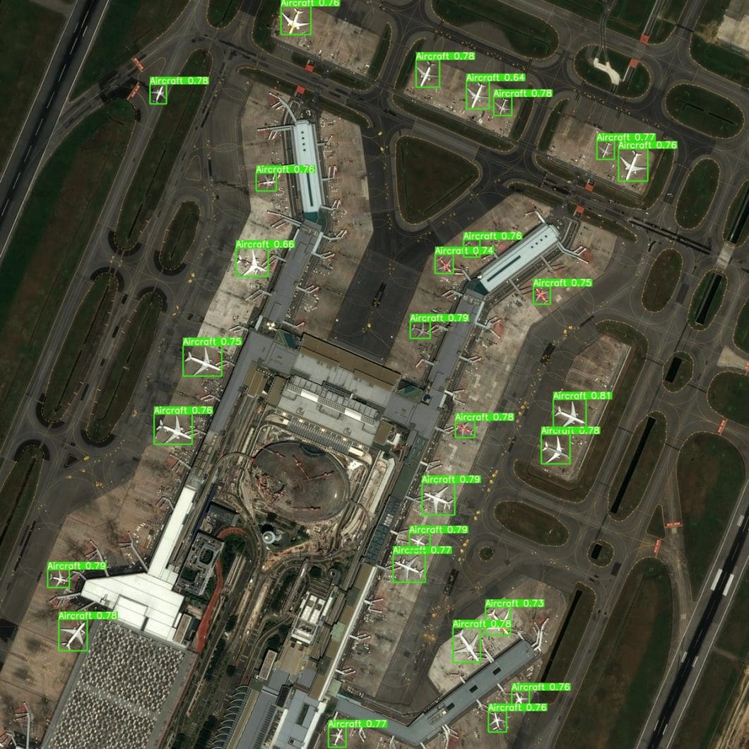
- Object Detection: When the goal is to recognize objects in image or video data, semi-supervised learning can be used to increase deep learning model performance.
- Image Segmentation: Semi-supervised learning can be used to improve models that classify each pixel in an image into one of several pre-defined classes.
- Anomaly Detection: In pattern recognition, semi-supervised learning can be used to make observations that do not conform to expected behavior.
- Data Imputation: Another use case includes models whose goal is to fill in missing values or estimate unknown values.
What are Popular Semi-supervised Learning Techniques?
Some popular techniques used in semi-supervised learning include self-training, co-training, and multi-view learning.
- Self-training involves training a model on the labeled data and then using it to label the unlabeled data. The labeled data is then augmented with the newly labeled data, and the process is repeated until convergence. This technique can be used for a variety of tasks, including image classification, natural language processing, and anomaly detection. Read more about self-training further below in this article.
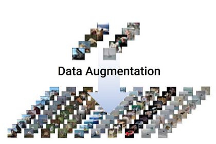
- Co-training requires the training of two models on different views of the data and then using them to label the unlabeled data. Through data augmentation, the annotated data can be expanded, a process that is repeated until convergence. This technique is particularly useful when the data has multiple representations, such as text and images.
- Multi-view learning is the training of a model that can make use of multiple views of text or image data. This model learns to make use of the complementary information present in different views to improve performance.
- Multi-task learning is used to learn multiple related tasks simultaneously and to leverage the shared information across tasks to improve performance.
- Generative Adversarial Networks (GANs) are a class of models that can be used for semi-supervised learning. GANs use the training of a generator to produce new samples that are similar to the labeled samples, and a discriminator to distinguish between the labeled and generated samples.
Differences Between Semi-supervised and Self-supervised Learning
Semi-supervised learning and self-supervised learning are both types of machine learning that utilize both labeled and unlabeled data to train models. However, there are some key differences between semi- and self-supervised learning:
- Labeled data: In semi-supervised learning, the model is trained on a small set of labeled data and a large set of unlabeled data. In contrast, self-supervised learning does not require any labeled data and only uses unlabeled data.
- Pretext task: Self-supervised learning requires the model to be trained on a “pretext task,” which is a task created by the researcher that requires the model to learn useful features from the data. Semi-supervised learning does not require the model to be trained on a pretext task.
- Transfer learning: Self-supervised learning is often used to learn useful features that can be transferred to other tasks. On the other hand, semi-supervised learning is used to improve the performance of a specific task.
- Purpose: Semi-supervised learning is advantageous when annotated ground data for training for a characteristic task is difficult or costly to obtain. Self-supervised learning is useful when the goal is to learn useful features that can be transferred to other tasks.
The Semi-supervised Scenario
Defining the Scenario
How is a semi-supervised scenario defined? How does this definition differentiate it from other data scenarios? In a fully supervised approach, we can rely on a completely labeled dataset, while we only have a limited number of data points in a semi-supervised approach.
While the training sample is assumed to be drawn uniformly in other methods, this is not the case for semi-supervised machine learning methods. The context of semi-supervised learning methods is defined instead by the union of two given sets with non-uniform data.
Semi-Supervised Model Dataset
Semi-supervised models have one labeled and unlabeled dataset, whereas the unlabeled dataset has a distribution that does not dramatically differ from the labeled dataset in terms of balance between classes. Unlabeled samples in semi-supervised learning datasets are supposed to be missing at random without any correlation with the label distribution. For example, we cannot have 10% of the dataset consisting of one class while the rest belongs to another.
There are generally no restrictions on the number of data points among datasets. However, semi-supervised problems often arise when the number of unlabeled points is a great margin larger than the number of data points in the labeled set. The complexity contributed by using semi-supervised models as opposed to supervised ones is justified when the number of data points of the labeled set is lower than the amount of unlabeled data.
This is a common condition because most datasets constitute a situation where there is a vast amount of unlabeled data and a small set of labeled data. This is because large, detailed, accurately annotated datasets can be expensive and include a limited subset of possibilities for classes and diversity.
Transductive Learning
Transductive learning refers to the approach used when a semi-supervised model aims to find labels for unlabeled samples. In transductive learning, instead of being interested in modeling the entire distribution p(y|x) (probability of y given x), we are only interested in finding the distribution of the unlabeled points.
Transductive learning can be time-saving and is preferable when the goal is oriented toward improving our knowledge about the unlabeled dataset. However, because this scenario implies that the knowledge of the labeled dataset can improve our knowledge of the unlabeled dataset, it is not ideal or usable for causal processes.
Inductive Learning
Inductive learning considers all data points and tries to determine a complete function where y = f(x) can map both labeled and unlabeled data points to their respective labels. This method is more complex than transductive learning and proportionately requires more computational time.
Semi-supervised Assumptions
Semi-supervised learning is not guaranteed to improve a supervised model. A few wrong choices could lead to an evolution where performance continuously worsens. It’s possible, however, to state some fundamental assumptions that are required for semi-supervised learning to work properly.
These assumptions are empirical mathematical observations that justify otherwise arbitrary choices of approach. The two assumptions we will discuss are the smoothness and cluster assumptions.
Smoothness Assumption
In a nutshell, the semi-supervised smoothness assumption states that if two points (x1 and x2) in a high-density region are close, then so should their corresponding outputs (y1 and y2). By the transitive property, this assumption entails that when two points are linked by a path of high data density (for example, belonging to the same cluster), then their outputs are also likely to be close together. When they are separated by low-density regions, their outputs do not have to be as close.
For semi-supervised learning, the knowledge of p(x) (probability of x) that one gets by analyzing unlabeled data has to carry information that is useful in the inference of p(y|x). When this is not the case, applied semi-supervised learning techniques will not yield significant or existing improvement over supervised learning. A more negative outcome would be where unlabeled data degrades accurate predictions by misguiding the inference.
A generalization of the smoothness assumption useful for semi-supervised learning is known as the “semi-supervised smoothness assumption.” While in supervised cases, the output of the machine learning model varies with the distance, we also take into account the input density in semi-supervised cases. The assumption here would be that the label function is smoother in high-density regions than in low-density regions.
Definition of “smoothness”: If an x input produces a y output, then an input close to x would produce an output proportionately close to y. The accuracy of predicting correctly increases with increasing smoothness.
Cluster Assumption
The cluster assumption, in essence, states that if points are in the same cluster, they are likely to be of the same class. Clusters are high-density regions, so if two points are close together, they’re likely to belong to the same cluster, and thus, their labels are likely to be the same.
Low-density regions are spaces of separation between high-density regions, so samples belonging to low-density regions are more likely to be boundary points rather than belong to the same class as the rest of the cluster.
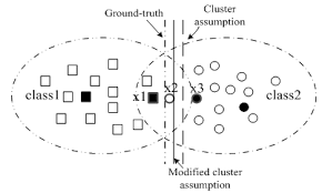
Therefore, two points from low-density clusters can be of different classes. The cluster assumption is reasonable due to the characteristics of classes: if there is a densely populated cluster of objects, it may be unlikely that they are of different classes.
In a semi-supervised scenario, we are not given all the labels of data points but do have the labels for a few. We couldn’t know the label of a point belonging to a high-density region, but if that data point is close to a given labeled point, we can predict the label of that test sample.
This works when the unlabeled data point is close enough to the labeled data point so that we can view all the points in a ball where they have the same average density. The same densities allow us to predict the label of the unknown data point.
By this logic, moving to low-density regions causes the process to increase in complexity because, as we discussed previously, low-density data points can be boundary points and thus be close together yet have different labels.
Manifold Assumption
A manifold is a collection of points forming a certain kind of set or cluster. For example, if we drew three points on a flat sheet of paper and then crumpled that piece of paper into a ball, the points have gone from being located in 2 dimensions to 3.
In machine learning, a manifold is an object of a certain dimensionality that is embedded in a higher-dimensional space. In the context of our paper, the manifold is the collection of three points on a 2D plane within the new 3D space.
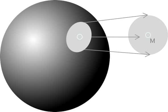
For instance, in the image above, there is a 2-dimensional plane within a 3-dimensional plane, where the 2-dimensional shape M is the manifold obtained from the general larger spherical surface. M, in this case, would contain the data points we are interested in.
The manifold assumption states that the data used for semi-supervised learning lies on a low-dimensional manifold embedded in a higher-dimensional space. Therefore, data points that follow this assumption need to be densely sampled. In other words, the data should, instead of coming from every part of the possible space, come from relatively low-dimensional manifolds.
The manifold assumption implies that all instances of a universal family (ex., images) are clustered into separate subspaces where some are semantically valid while most others are noisy (and thus negligible). Because we’ve now defined and provided overviews of the concepts surrounding semi-supervised scenarios, we can start discussing specific semi-supervised algorithms that rely on both labeled and unlabeled datasets to perform more accurate classifications than supervised approaches.
Generative Gaussian Mixture
Generative Gaussian Mixture is an inductive algorithm for semi-supervised classification. It is used for modeling the conditional probability of x and y given both labeled and unlabeled data sets and is especially helpful when the goal is to find a model explaining the structure of existing data points. In addition, the algorithm can output the probability of new data points.
Generative Gaussian Mixture aims to model the data-generating process using a sum of weighted Gaussian distributions. The model is generative, meaning the probability distribution of data is modeled to perform pattern recognition. The structure of the algorithms allows us to cluster the given datasets into well-defined regions (Gaussians) and output the probability of new data points belonging to each of the classes.
What is Self-Training?
Self-training is an approach to semi-supervised classification that involves the application of both the smoothness and cluster assumptions discussed previously. Therefore, self-training is also known as self-labeling or decision-directed learning.
In general, self-training is a good option and a valid decision when the labeled dataset contains plenty of information about the data-generating process and when the unlabeled sample is assumed to be responsible just for fine-tuning the algorithm at hand.
However, self-training is not an ideal choice when these conditions are not met because it largely depends on the composition of the labeled sample.
In each step of self-training, a part of the unlabeled data points are labeled according to the current decision function, and the supervised model is retrained using its predictions as additional labeled points.
How Self-Training Works
Self-training algorithms train a model to fit pseudo labels predicted by another previously learned supervised model. These algorithms have been successful in the past for learning using neural networks with unlabeled data.
Self-training consists of a few key points:
- Labeled data instances are split into train and test sets, where a classification algorithm is trained on the labeled training data. All data points are evaluated, and each prediction is represented using a confidence vector.
- The first K values associated with the largest confidences are selected and added to the labeled dataset.
- The classifier predicts class labels for the labeled test data instances, and classifier performance is evaluated using metrics of choice.
- The classifier is retrained using the newly labeled dataset.
Self-training leverages the structure of the labeled dataset to discover a suitable separation hypersurface. After this process, the unlabeled sample is evaluated, and the points classified with sufficiently large confidence are included in the new training set- this procedure is replicated until every data point is classified.
What’s Next
There are multiple facets to semi-supervised learning. Semi-supervised learning methods for computer vision have also been developing into advanced processes at rapid rates during the past few years.
In addition to the topics discussed here, semi-supervised learning also includes co-training, support vector machines, and likelihood estimation, both of which expand semi-supervised learning into a deeper subset of machine learning.
If you enjoyed this article, we suggest you also read:
- Self-Supervised Learning: What It Is, Examples and Methods for Computer Vision: frameworks discussed include Pre-trained Language Models (PTM), Generative Adversarial Networks (GAN), Autoencoder and its extensions, Deep Infomax, and Contrastive Coding – extensions of supervised learning, involved in machine learning along with semi-supervised learning.
- YOLOv3: Real-Time Object Detection Algorithm and YOLOv7 for computer vision and image detection.
- Introduction to Federated Learning: A new learning paradigm where statistical methods are trained at the edge in distributed networks.
- Read an introduction to Machine Vision
