YOLOv10 is the latest advancement in the YOLO (You Only Look Once) family of object detection models, known for real-time object detection. The YOLOv10 model pushes the performance-efficiency boundaries, building on the success of its predecessors. The new exciting enhancements promise to transform real-time object detection across various applications.
Researchers have conducted extensive experiments on the YOLO models, achieving notable progress. However, YOLOv10 aims to advance previous variations’ post-processing and model architecture. The result is a new generation of the YOLO series for real-time end-to-end object detection.
Get ready for a deep dive into YOLOv10. We will examine the architectural modifications, compare its efficiency with other YOLO models, uncover its practical uses, and demonstrate how to apply it for inference and training on your data.
About us: Viso Suite provides computer vision infrastructure for enterprises. As the only end-to-end solution, Viso Suite consolidates the entire application pipeline into a robust interface. Learn more about how companies worldwide are using Viso Suite for everyday business solutions.
YOLOv10: An Evolution of Object Detection
The YOLO series has been predominant over the years in the field of real-time object detection. Each YOLO model comes in multiple sizes with a different balance of accuracy and speed. Below are the usual sizes for a YOLO model, including the latest YOLOv10.
- YOLO-N (Nano)
- YOLO-S (Small)
- YOLO-M (Medium)
- YOLO-B (Balanced)
- YOLO-L (Large)
- YOLO-X (X-Large)
Object detection, especially in real-time has always been an important area of research in computer vision. The purpose of object detection in real-time is to locate and identify objects in an image under low latency. Researchers typically employ variations of a Convolution Neural Network (CNN) like R-CNN (Regional CNN), Fast R-CNN, Faster R-CNN, and Mask R-CNN.
However, YOLO models utilize a more complex architecture than that, offering a balance between performance and efficiency for real-time object detection. Let’s recap these basics before diving into the specifics of YOLOv10.
Background
The earliest object detection method was the sliding window approach where a fixed-size bounding box moves across the image until we find the object of interest. As this is resource-intensive, researchers developed more efficient approaches, such as Faster R-CNN, one of the earliest approaches moving toward real-time object detection.
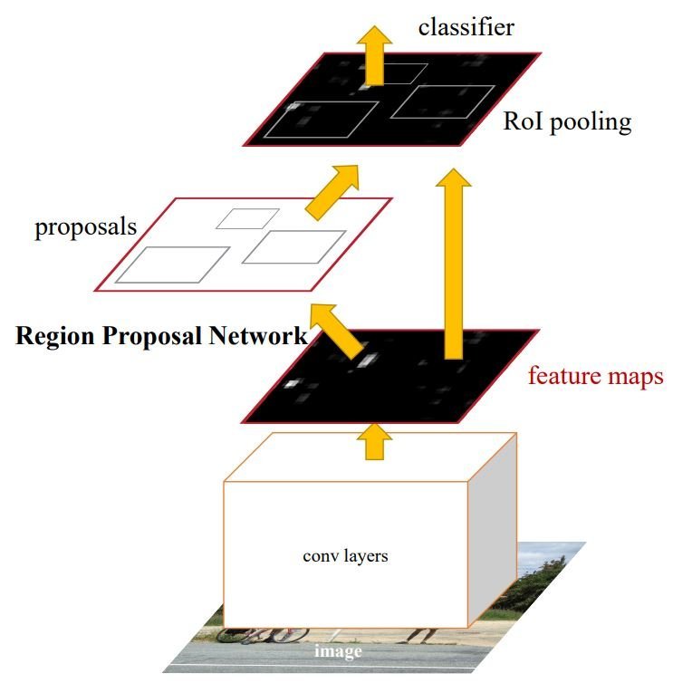
The idea behind Faster R-CNN is to use R-CNN which aims to optimize the sliding window approach with a region proposal network. This algorithm would propose bounding boxes where the object is more likely to be. Then Convolutional layers extract feature maps that are used to classify the objects within the bounding boxes. Additionally, Faster R-CNN includes optimization to increase speed and efficiency.
However, the YOLO models come with a different approach in mind. These models utilize a single-shot method, where both detection and classification happen in one step. YOLO models, including YOLOv10, frame object detection as a regression problem, where a single neural network predicts the bounding boxes and the classes in one evaluation.

The YOLO detection system works in a pipeline of a single network, thus it is optimized for detection performance.
- The pipeline first resizes the image to the input size of the YOLO model.
- Runs a Convolutional Neural Network on the image.
- The pipeline then utilizes Non-max suppression (NMS) to optimize the CNN’s detections by applying confidence thresholding.
Non-maximum suppression (NMS) is a technique used in object detection to remove duplicate bounding boxes and select only the relevant ones. By tuning this postprocessing technique and other techniques like optimization, data augmentation, and architectural changes, researchers create different variations of YOLO models. As we’ll see later, the YOLOv10’s most notable evolution is related to the NMS technique.
Benchmarks
To understand the advancements in YOLOv10, we will start by comparing its benchmark results to those of previous YOLO versions. The two main performance measures used with real-time object-detection models are usually average precision (AP) or mAP (mean AP), and latency. We measure those metrics on benchmark datasets like the COCO dataset.
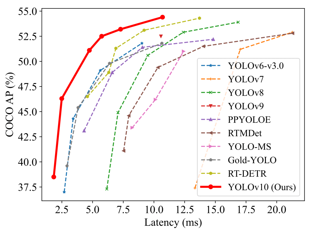
While this comparison shows only metrics like latency and AP, we can see how the YOLOv10 model significantly improves those measures. We need to look at a more detailed comparison to understand the full picture. This comparison will show other metrics to inspect the areas where YOLOv10 excels.
| Model | Params (M) | FLOPs (G) | APval (%) | Latency (ms) | Latency (Forward) (ms) |
|---|---|---|---|---|---|
| YOLOv6-3.0-S | 18.5 | 45.3 | 44.3 | 3.42 | 2.35 |
| YOLOv8-S | 11.2 | 28.6 | 44.9 | 7.07 | 2.33 |
| YOLOv9-S | 7.1 | 26.4 | 46.7 | – | – |
| YOLOv10-S | 7.2 | 21.6 | 46.3 / 46.8 | 2.49 | 2.39 |
| YOLOv6-3.0-M | 34.9 | 85.8 | 49.1 | 5.63 | 4.56 |
| YOLOv8-M | 25.9 | 78.9 | 50.6 | 9.50 | 5.09 |
| YOLOv9-M | 20.0 | 76.3 | 51.1 | – | – |
| YOLOv10-M | 15.4 | 59.1 | 51.1/51.3 | 4.74 | 4.63 |
| YOLOv8-L | 43.7 | 165.2 | 52.9 | 12.39 | 8.06 |
| YOLOv10-L | 24.4 | 120.3 | 53.2 / 53.4 | 7.28 | 7.21 |
| YOLOv8-X | 68.2 | 257.8 | 53.9 | 16.86 | 12.83 |
| YOLOv10-X | 29.5 | 160.4 | 54.4 | 10.70 | 10.60 |
As shown in the table, we can see how the YOLOv10 achieves state-of-the-art performance across various scales. YOLOv10 compared to baseline models like the YOLOv8 has a range of improvements. The S/ M/ L/ X sizes achieve 1.4%/0.5%/0.3%/0.5% AP improvement with 36%/41%/44%/57% fewer parameters and 65%/ 50%/ 41%/ 37% lower latencies. Importantly, YOLOv10 achieves superior trade-offs between accuracy and computational cost.
These improvements against other YOLO variations like the YOLOv9, YOLOv8, and YOLOv6, indicate the effectiveness of the YOLOv10’s architectural design. Next, let’s inspect and explore the architectural design of YOLOv10.
The Architecture Of YOLOv10
The architecture design in YOLO models is a fundamental challenge because of its effect on accuracy and speed. Researchers explored different design strategies for YOLO models, but the detection pipeline of most YOLO models remains the same. There are two parts to the pipeline.
- Forward process
- NMS postprocessing
Furthermore, YOLO architecture design usually consists of 3 main components.
- Backbone: Used for feature extraction creating a representation of the image.
- Neck: This component, introduced in YOLOv4, is the bridge between the backbone and the head. It combines features across different scales from the extracted features.
- Head: This is where the classification happens, it predicts the bounding boxes and the classes of the objects.
With that in mind, we will look at the key improvements and architectural design of the YOLOv10.
Key Improvements
Since YOLOs frame object detection as a regression problem, the model divides the image into a grid of cells.
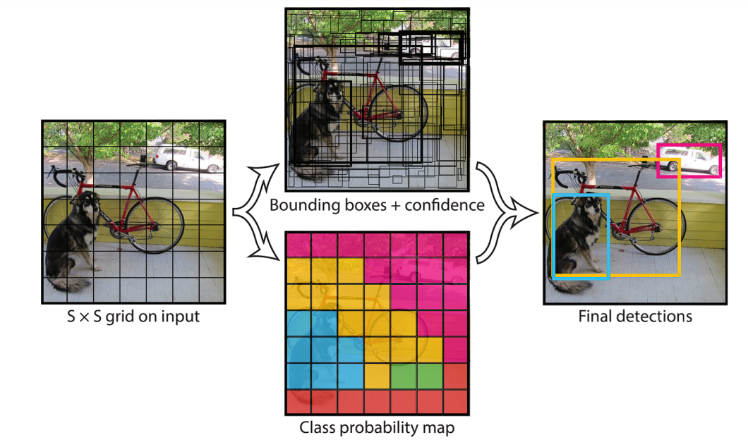
Each cell is responsible for predicting multiple bounding boxes. In YOLOs, each ground-truth object (the actual object in the training image) is associated with multiple predicted bounding boxes.
This one-to-many label assignment strategy has shown strong performance but requires Non-Maximum Suppression (NMS) during inference. NMS relies on Intersection over Union (IoU), a metric to calculate the overlap between the predicted bounding box and the ground truth. By setting an IoU threshold, NMS can filter out redundant boxes.
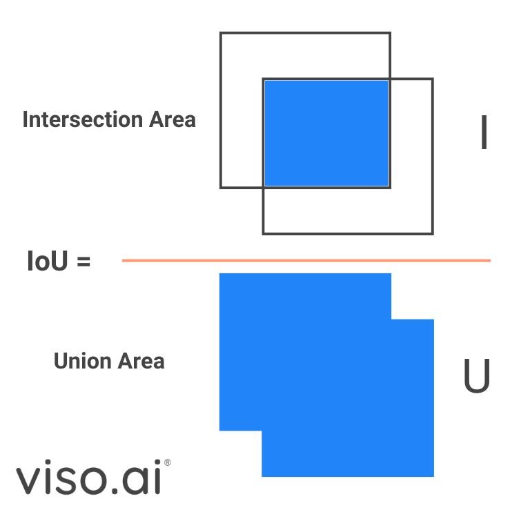
However, this post-processing step slows down the inference speed, preventing YOLOs from reaching their optimal performance. The YOLOv10 eliminates the NMS postprocessing step with NMS-Free training. The researchers utilize a consistent dual assignments training method that efficiently reduces the latency.
Consistent dual assignment allows the model to make multiple predictions on an object, with a confidence score for each. During inference, we can select the bounding box with the highest IOU or confidence, reducing inference time without sacrificing accuracy.
Additionally, YOLOv10 includes improvements in the optimization and architecture of the model.
- Holistic Design: This refers to the optimization done to various components of the model, the holistic approach maximizes the efficiency and accuracy of each. We will delve deeper into the specifics of this design later.
- Improved Architecture and Capabilities: This includes changes to the convolutional layers, and adding partial self-attention modules to enhance efficiency without risking computational cost.
Next, we will look at the components of the YOLOv10 model, exploring the improvements.
Components of YOLOv10
YOLOv10 components build upon the success of previous YOLO versions, retaining much of their structure while introducing key innovations. During training, YOLOs usually use a one-to-many assignment strategy which needs NMS postprocessing. Other previous works have explored things like one-to-one matching which assigns only one prediction to each object, thus eliminating NMS, but this introduced additional inference overhead.
The YOLOv10 introduces the dual-label assignment and consistent matching metric. This combines the best of the one-to-one and the one-to-many label assignments and achieves high performance and efficiency.
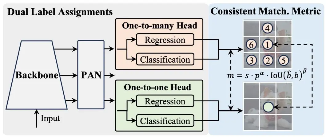
As shown in the figure above, the YOLOv10 adds a one-to-one head to the architecture of YOLOs. This head retains the same structure and optimization as the original one-to-many head.
- While training the model, both heads are jointly optimized giving the backbone and the neck rich supervision.
- The rich supervision comes from the ability of the one-to-many assignment strategy to allow the model to consider multiple potential bounding boxes for each ground truth object. This gives the backbone and neck models more information to learn from.
- The consistent matching metric optimizes the one-to-one head supervision to the direction of the one-to-many head. A metric measures the IOU agreement between both heads and aligns their predictions.
- During inference, the one-to-many head is discarded and we use the one-to-one head to make predictions. YOLOv10 also adopts the top-one selection method, ultimately giving it less training time and no additional inference costs.
The backbone and neck are also important components in any YOLO mode. Specifically, in YOLOv10 the researchers employed an enhanced version of CSPNet to do feature extraction. They also used PAN layers to combine features from different scales within the neck.
Holistic Design-Efficiency-Driven
The YOLOv10 aims to optimize the components from efficiency and accuracy perspectives. Starting with the efficiency-driven model design, the YOLOv10 applies optimization to the downsampling layers, the basic building block stages, and the head.
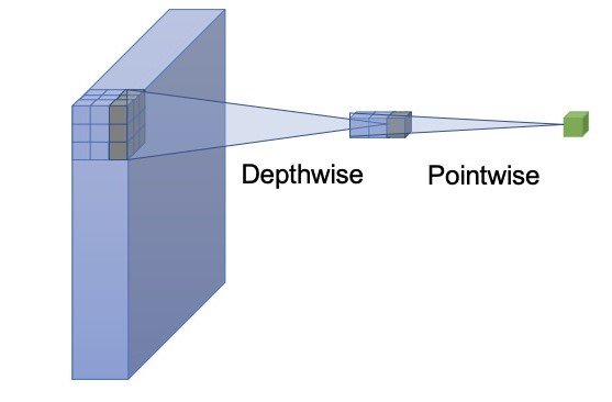
The first optimization is the lightweight classification head using depth-wise separable convolution. YOLOs usually use a regression and a classification component. A lightweight classification head will reduce inference time and not greatly hurt performance. Depth-wise separable convolution consists of a depthwise and a pointwise network, the one adopted in YOLOv10 has a kernel size of 3×3 followed by a 1×1 convolution.
The second optimization is the spatial-channel decoupled downsampling. YOLOs typically use regular 3×3 standard convolutions with a stride of 2. Instead, the YOLOv10 uses the pointwise convolution to adjust the channel dimensions and the depthwise for spatial downsampling. This approach separates the two operations leading to reduced computational cost and parameter count.
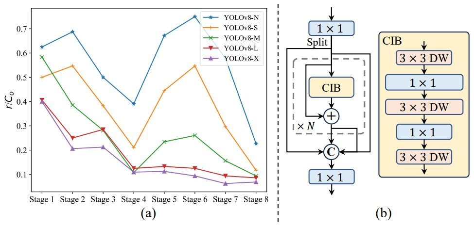
Furthermore, the YOLOv10 utilizes a third optimization for efficiency, the rank-guided block design. YOLOs usually use the same basic building blocks for all stages. Thus, the researchers behind YOLOv10 introduce an intrinsic rank metric to analyze the redundancy of model stages.
The analyses show that deep stages and large models are prone to more redundancy, part (a) of the figure above. This causes inefficiency and suboptimal performance.
To address this, they introduce the rank-guided block design:
- Compact inverted block (CIB): Uses cost-effective depthwise convolutions for spatial mixing and pointwise convolutions for channel mixing, part (b) of the figure above.
- Rank-guided block allocation: Sort all stages of a model based on their intrinsic ranks in ascending order. Additionally, they replace redundant blocks with CIBs in stages where it doesn’t affect performance.
Holistic Design-Accuracy-Driven
Efficiency and accuracy are the biggest trade-offs in object detection, but the YOLOv10 holistic approach minimizes this trade-off. The researchers explore large-kernel convolution and self-attention for the accuracy-driven design, boosting performance with minimal costs.
The first accuracy-driven optimization is the large-kernel convolution. Using large kernel convolutions can enhance the model’s receptive field improving object detection. However, using those convolutions in all stages can cause problems detecting small objects or be inefficient in high-resolution stages.
Therefore, the YOLOv10 introduces using large-kernel depthwise convolutions in compact inverted block (CIB), only in the deeper stages and with small model scales. Specifically, the researchers increase the kernel size from 3×3 to 7×7 in the second depthwise convolution of the CIB.
Additionally, they use the structural reparameterization technique by introducing an additional 3×3 depthwise convolution branch which mitigates potential optimization issues and retains the benefits of smaller kernels.
This optimization enhances the model’s ability to capture fine details and contextual information without sacrificing efficiency or cost during inference.
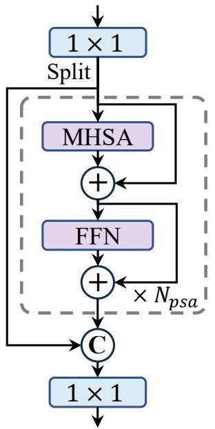
Lastly, the YOLOv10 employs an additional accuracy-driven optimization, the partial self-attention (PSA). Self-attention is widely used in visual tasks for its powerful global modeling capabilities but comes with high computational costs. To address this, the researchers of YOLOv10 introduce an efficient design for the partial self-attention module.
Specifically, they evenly divide the features across channels into two parts and only apply self-attention (NPSA blocks) to one part. Additionally, they optimize the attention mechanism by reducing the dimensions of query and key and replacing LayerNorm with BatchNorm for faster inference. This reduces cost and keeps the global modeling benefits.
Furthermore, PSA is only applied after the stage with the lowest resolution to control the computational overhead, leading to improved model performance.
Implementation And Applications Of YOLOv10
The accuracy and efficiency-driven design is an evolutionary step for the YOLO family. This comprehensive inspection of components resulted in YOLOv10, a new generation of real-time, end-to-end object detection models.
While real-time object detection has existed since Faster R-CNN, minimizing latency has always been a key goal. The latency of a model is a crucial factor in determining its practical applications. High-integrity applications need to have optimal performances in efficiency and accuracy, and that is what YOLOv10 gives us.
We will explore the YOLOv10 code, and then look at how it can evolve real-world applications.
YOLOv10 Inference-HuggingFace
Most YOLOs are easily implemented with Python code through the Ultralytics library. This library gives us the option to train and fine-tune YOLO models on our data, or simply run inference. However, YOLOv10 is still not fully integrated into the Ultralytics library. We can still try the YOLOv10 and use its code through the available Colab notebook or the HuggingFace spaces.
Let’s start by checking out the HuggingFace space.
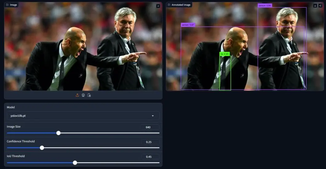
Using one of the examples available, we can see how the YOLOv10 can quickly generate predictions. We can also use the available options to test and try various settings and see how they differ. In the example above, we are using the YOLOv10-base model, with an image size of 640×640. Additionally, we have the confidence and IoU thresholds.
While the IoU threshold won’t hold many benefits during inference, we have learned its importance during training. On the other hand, the confidence threshold is useful during inference, especially for complex images, a higher value makes more accurate predictions but overall fewer predictions, and the opposite is true.
Inference-Command line Interface (CLI)
Furthermore, we can delve into the code for YOLOv10 through the Colab notebook. The notebook tutorial is pretty clear and gives you options like running inference using the command line interface (CLI), or the Python SDK, as well as an option to train on custom data.
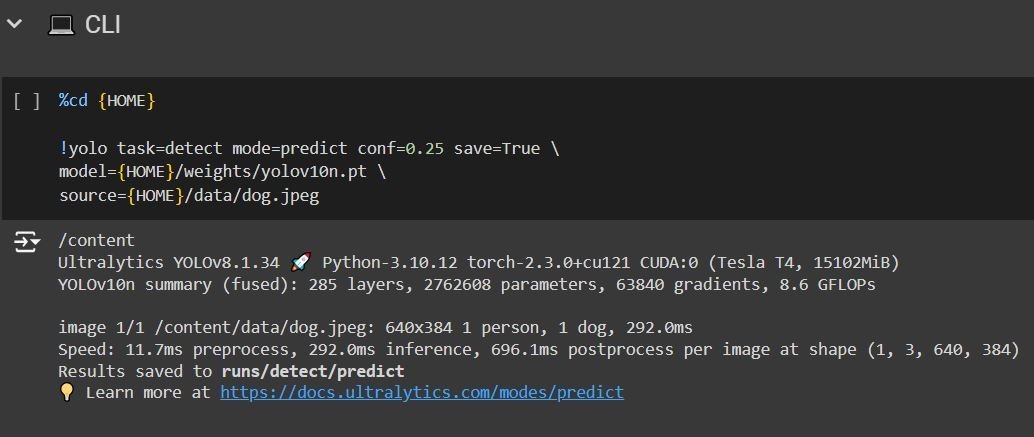
After running all the previous code blocks, you will have to run them as they are because they provide the necessary setup to use YOLOv10. Now you can try the CLI inference, the above code uses the yolov10-nano model, uses a confidence threshold of 0.25, and uploads an image from the data provided by the notebook.
If we want to make inferences on different model sizes, a custom image, or adjust the confidence threshold we can simply do:
%cd {HOME} #Navigate to home directory
!yolo task=detect mode=predict conf=0.25 save=True \ # using the !yolo command to run cli inference. Define the task as prediction, and use the predict model, adjust conf value as needed.
model={HOME}/weights/yolov10l.pt \ # Changing the letter after YOLOv10 will change the model size. Model sizes are discussed earlier in the article.
source=/content/example.jpg # Upload Image directly to Colab on the left handside, or mount the drive and copy image path
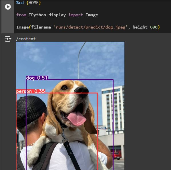
In the next code block, we can show the result prediction using the Python display library, the “filename” variable indicates where the result images are saved (notice that we use save=True in the CLI command).
Inference-Python SDK
The code block after that shows the usage of YOLOv10 using the Python SDK:
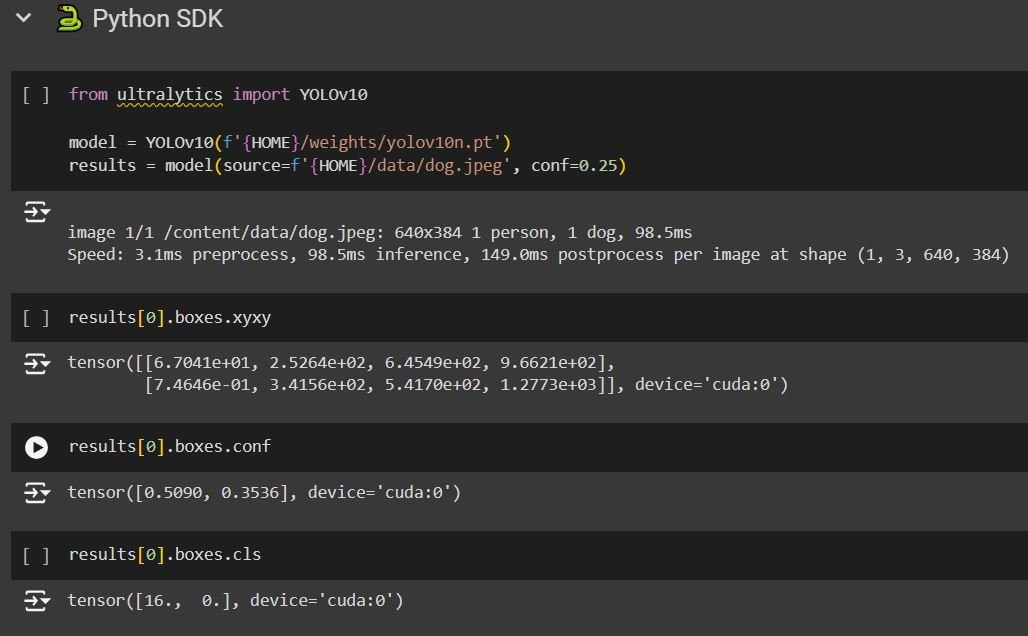
The SDK inference provides us with additional information regarding the prediction. We can see the coordinates of the boxes, the confidence, and lastly “boxes.cls” representing the number of the category (class) detected.
This code is also adjustable, so you can use the model size and the image you want. The next code block shows how we can display the prediction using the “supervision” library, which will also show information like the postprocessing and preprocessing speed, the inference speed, and the category names.
With this, we have concluded the usage of YOLOv10 through code and HuggingFace, the notebook provided in the official YOLOv10 GitHub is quite useful and the tutorial within will guide you through the process. However, training the YOLOv10 requires extra effort to create your own dataset, and iterate with the training process.
Now let’s look at ways we can use these enhancements of the YOLOv10 in real-world applications.
Real-World Applications of YOLOv10
YOLOv10’s efficiency, accuracy, and lightweight make it suitable for a variety of applications, perhaps replacing previous YOLO models in most real-time detection applications. Those new capabilities are pushing the boundaries of what’s possible in computer vision.
- Object Tracking: The latency improvement in YOLOv10 makes it very suitable for use cases that need object-tracking in video streams. Applications range from sports analytics (tracking players and ball movement) to security surveillance (identifying suspicious behavior).
- Autonomous Driving: Object detection is the core of self-driving cars. The ability of an object detection model to detect and classify objects on the road is essential for this use case. YOLOv10’s speed and accuracy make it a prime candidate for real-time perception systems in autonomous vehicles.
- Robot Navigation: Robots equipped with YOLOv10 can navigate complex environments by accurately recognizing objects and obstacles in their paths. This enables applications in manufacturing, warehouses, and even household chores
- Agriculture: Object detection can be crucial for crop monitoring (identifying pests, diseases, or ripe produce) and automated harvesting. YOLOv10’s accuracy and lightweight make it well-suited for these applications.
While those are only a few applications, the possibilities are endless for YOLOv10. A new age of real-time object detection is coming, and YOLOv10 might be the start.
What’s Next For YOLOv10?
YOLOv10 is a significant leap forward in the evolution of real-time object detection. Its innovative architecture, clever optimization, and remarkable performance make it a valuable tool for a variety of applications.
But what does the future hold for YOLOv10, and the broader field of real-time object detection? One thing is clear: innovation doesn’t stop here. Expect to see even more refined architectures, streamlined training processes, and a wider range of applications for this versatile technology.
YOLOv10 is a significant milestone, but it’s just one step in the ongoing evolution of object detection. We’re excited to see where this technology takes us next!
Recommended Reads for YOLOv10
If you want to know more about the older models and how Yolov10 is different from them, read our articles below:
- YOLOv3: Real-Time Object Detection Algorithm (Guide)
- YOLOv5 Is Here! Is It Real or a Fake?
- YOLOv7: A Powerful Object Detection Algorithm
- A Guide to YOLOv8
- YOLOv9: Advancements in Real-time Object Detection
- YOLOX Explained: Features, Architecture and Applications
- YOLOR : You Only Learn One Representation


